


Document Actions
gvSIG-Desktop 1.10. User Manual
- Viewing and accesing data
- Layer data source
- Consulting tools
- Information tool
- Herramienta de información rápida
- Measuring areas
- Measuring distances
- Catalogue. Searching for geodata
- Gazetteer
- Hiperenlace avanzado
- Navigation tools
- Navigating around / Exploring the view
- Configuring the locator map
- Centring the view on a point
- Locate by attribute
- Load data
- Geographical data
- Introduction
- Vectorial
- Adding a layer from a disk file
- Adding a layer using the WFS protocol
- Introduction
- Connecting to the server
- Accessing the service
- Selecting 'Layers'
- Selecting 'Attributes'
- 'Options' tab
- Filter
- Adding the layer to the view
- Modifying the layer's properties
- Filtrado por área
- Adding a layer using the ArcIMS vectorial
- Introduction to ArcIMS
- Connecting to image services
- Adding a layer using the ArcIMS protocol
- Add layer using the arcIMS protocol
- Connecting to the server
- Accessing the service
- Selecting layers
- Adding the layer to the view
- Points to remember about spatial reference systems
- Modifying the layer's properties
- Information about scale limits
- Attribute information requests
- Connecting to geometry services
- Adding a geometry layer
- ArcIMS symbols
- Symbols
- Legends
- Working with the layer
- geoDB Extension (database manager)
- Introduction
- The spatial connection database manager
- Adding a geoDB layer to the view
- Exporting a gvsig layer to a spatial database
- Oracle spatial
- Introduction
- Metadata
- Data types
- Coordinate systems in Oracle
- Notes on reading geometries
- Transferring a layer from gvSIG to Oracle
- ArcSDE
- Adding an Event layer
- Introduction
- Adding an event layer from a table
- Adding an event layer from a table associated with a layer in the view
- Coordinate Reference Systems
- Raster
- Adding a layer from a disk file
- Adding a layer using the WMS protocol
- Connecting to the service
- Accessing the service
- Selecting 'Layers'
- Selecting 'Styles' for the WMS server layers
- Selecting values for a WMS layer's 'Dimensions'
- Selecting the format, spatial system and/or transparency
- Adding the layer to the view
- Modifying the layer's properties
- Adding a layer using the WCS protocol
- Accessing the service
- Selecting 'Coverages'
- Selecting the 'Format'
- Adding the layer to the view
- Modifying the layer's properties
- Adding orthophotos using the ECWP protocol
- Adding a layer using the ArcIMS raster
- Introduction to ArcIMS
- Connecting to image services
- Adding a layer using the ArcIMS protocol
- Add layer using the arcIMS protocol
- Connecting to the server
- Accessing the service
- Selecting layers
- Adding the layer to the view
- Points to remember about spatial reference systems
- Modifying the layer's properties
- Information about scale limits
- Attribute information requests
- Connecting to geometry services
- Adding a geometry layer
- ArcIMS symbols
- Symbols
- Legends
- Working with the layer
- Web Map Context
- Alphanumeric data
- Symbology
- Labelling
- Introduction
- Static labelling
- Advanced Labelling (user defined)
- Introduction
- Label features in the same way
- Label only when the feature is selected
- Define classes of features and label each differently
- Common options
- Single labelling
- Selection tools
- Selección de elementos
- Introduction
- Selecting by point
- Selecting by rectangle
- Selecting by polygon
- Selecting by layer
- Selecting by attributes
- Inverting the selection
- Clearing selection
- NavTable
Viewing and accesing data
Layer data source
Different types of cartographic information can be added to a view. Vector and raster files can be loaded. Each of these groups can contain a wide range of formats.
GIS data: The standard GIS format is the shape, which stores both spatial data and their attributes. A shape (also called “Shape file”) is actually three or more files with the same name and different extensions (even though in gvSIG it is handled as one file):
dbf: Table of attributes.
shp: Spatial data.
shx: Spatial data index.
From version 0.5 onwards, gvSIG also has the capacity to access the MySQL Spatial and PostGIS spatial data bases via a new driver which uses JDBC.
CAD data: These are vector drawing files which support the dxf and dgn formats. The CAD files may contain information on points, lines, polygons and texts. From version 0.4 onwards, gvSIG also allows access to the information contained in Autodesk’s 2000 dwg files.
WMS data (Web Mapping Service): gvSIG can be used to consult WMS data, i.e. data available on the web. WFS data (Web Feature Service): From version 0.5 onwards, gvSIG can be used to download WFS vector layers from servers that comply with the Open Geospatial Consortium (OGC) Standard.
WCS data (Web Coverage Service): From version 0.4 onwards, gvSIG allows access to remote information based on the OGC’s WCS protocol.
GML (Geography Markup Language): From version 1.0 onwards, gvSIG allows GML documents to be displayed and exported. Geography Markup Language (GML) is an XML format to transport and store geographic information whose design is based on specifications produced by the OGC group.
Images: gvSIG can display different raster images (tiff, jpg, ecw, mrsid, etc.). From version 0.4 onwards, gvSIG can save images which have been modified in these formats.
From version 0.5 onwards, “colour palette” (GIFs, 8-bit PNGs, etc.) raster files can be opened and raster files without georeferencing can also be opened. Moreover, this new version supports GIF, BMP y JPEG2000 formats.
Consulting tools
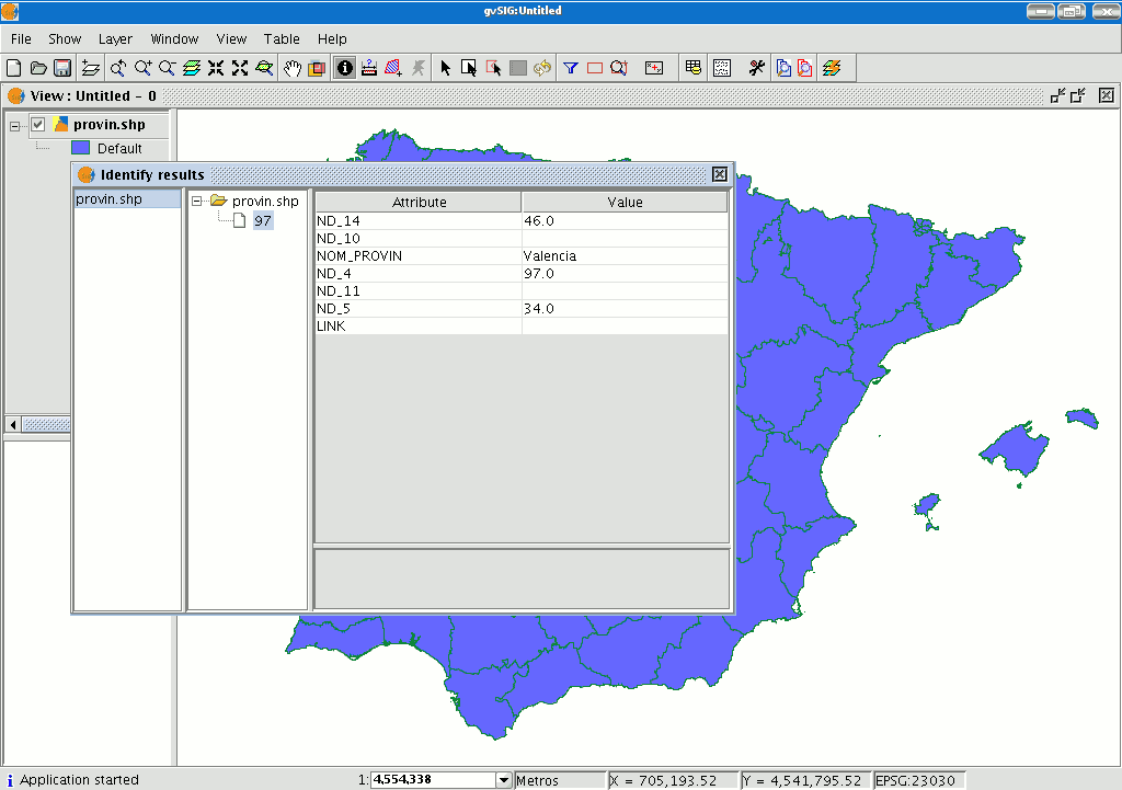
Information tool
You can access the information tool via the following button in the tool bar

or by going to the “View” menu bar, to “Query” and then to “Information”.
The “Information Tool” is used to obtain information about the map elements.
When you click on an element using this tool, gvSIG shows the selected element’s attributes in a dialogue window. However, the layer of the element you wish to identify must previously be activated.
Herramienta de información rápida
In gvSIG, this tool is used to quickly display available information when working with a view containing visible vector layers (including WFS layers, which are vector layers).
 Quick Info is enabled if vector layers are visible in the current view.
 Quick Info is disabled if no vector layers are visible in the current view.
With this tool you can select fields from vector layers visible in the current view. Information from these fields is displayed as you move the mouse cursor over the view. The tool works in combination with any other tools selected for the view.
You can access the Quick Info tool in two ways:
- Via the menu: View → Query → Quick Info
- Via the icon on the toolbar.
When the tool is selected a progress bar is displayed which shows the layers being loaded:
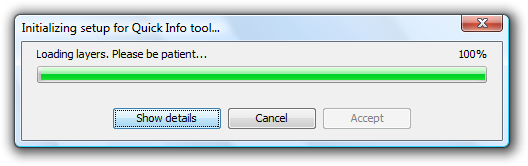
Progress bar for loading information
If there were no problems loading the information the Quick info field selection dialog is shown:
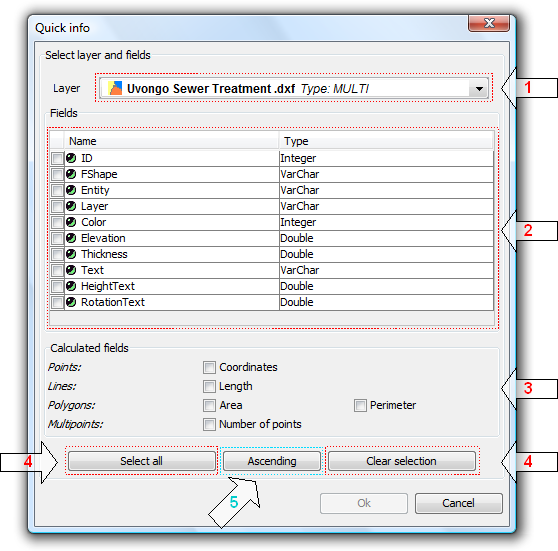
Dialog for the selection of fields
- Drop-down list for selecting vector layers. Lists the layers in the order that they appear in the TOC of the active view. The following information is shown:
Level of the Layer in the TOC: displays icons and grouping nodes  containing the layer. The last icon always represents the vector layer.
Name of the layer.
Type of geometry of the layer: five types of geometry layer are supported: point, line, polygon, multipoint, and multi (the latter may contain any of the above).
- List of Fields. Contains three columns:
- Selection box (checkbox): indicates whether or not to display the field information.
- Field Type + Field Name: the field type is represented by an icon as shown in the following table:
 The field type is simple.
- The field type is complex.
- Type of field: according to the SQL types.
- Calculated fields. List of checkboxes to select which geometry fields to calculate. These vary depending on the geometry of the layer:
- Point layer: point coordinates.
- Line layer: length of the line.
- Polygon layer: perimeter and area of the polygon.
- Multipoint layer: number of points.
- Multi-geometry layer: any of the above; the information will vary according to the selection and the nature of the geometry.
 The units of length and area are displayed using the measurement units of the View.
- Selecting / de-selecting all the fields in the layer. Select or de-select all the fields in the layer.
- Sort fields. Sort fields alphabetically in ascending or descending order, or according to the internal order of the layer (default).
After selecting the fields, click Ok to enable the tool in the current view. The Quick info tool works in combination with Quick info tools for other Views. Thus, when enabled, it combines with each active View to display information. The tool settings can be changed for each View and are linked to that View.
As the cursor is moved over the geometry of a layer, the information box showing the information is displayed and/or updated. This box disappears when the cursor no longer "points" to any geometry of the layer.
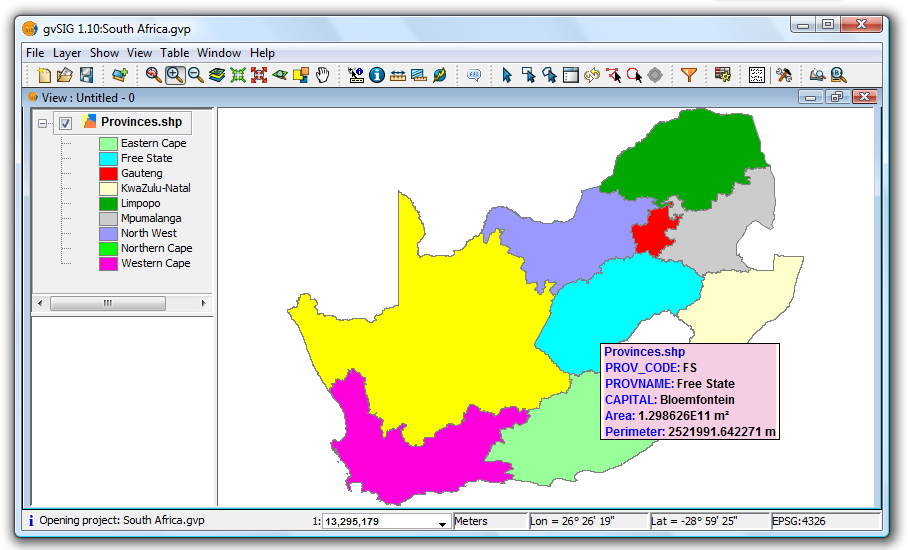
Example showing the display from the Quick info tool
If there is more than one geometry adjacent to the point indicated by the cursor then information is displayed about all of them, as distinguished by the unique internal identifier of the geometry.
Thus, the information is provided in the following order:
- Name of the layer.
- Information on the geometry (for each one):
ID: unique identifier of the geometry in the data source layer (optional, only visible if you have information on more than one geometry).
Selected fields: those fields selected to display layer information.
Optional fields: those calculated fields selected from the geometries of the layer.
 It should be noted that currently gvSIG adds the area and perimeter of islands to the geometry containing them.
Measuring areas
You can access this tool via the following button

or by going to the “View” menu and then to “Query” and “Measure area”.
This tool works in much the same way as “Measure distances”. Click on the point that represents the first polygon vertex that defines the area to be measured. Move the mouse and click on each new vertex until you reach the last one, then double click so that the application knows there are no more.
The calculation for the measured area appears at the bottom right of the view window.

Measuring distances

This tool provides information about the distance between two points. You can also access the tool by going to the “View” menu, to “Query” and then to “Measure distances”.

Firstly, make sure you have correctly defined the units of measurement (metres by default).
Remember that the units can be defined in the “Project manager” in the view properties or from the “View” menu and the “Properties” when working in a view.
You can use the measure distance tool by clicking on the mouse at the source point and dragging it to the destination point.
You can take as many measurements as you like. Double click on the last one to finish.
The calculation for the measured distance appears at the bottom of the view window. Both the distance of the last measured segment and the total distance are shown.
Catalogue. Searching for geodata
Introduction
The catalogue service allows you to search for geographic information on the Internet. gvSIG offers a user-friendly interface which allows you to find geodata and load it in the view, as long as the nature of the data allows this.
Connecting to a server
Before you can carry out a search, you will need to connect to a catalogue server. To access the wizard, you will first need to open a view and then click on the following button:

The first window of the catalogue opens. Input the required parameters to connect to a server. These include:
- The server address.
- The server protocol, which in the case of the catalogue can be:
- Z39.50: General information retrieval protocol.
- SRU/SRW: Variant of Z39.50.
- CSW: Catalogue protocol defined by the OGC in the “Catalogue Interface 2.0” specification.
- Data base name: You only need to indicate the data base you wish to connect to in the case of z39.50. If no value is input you will connect to the default data base.

Then click on the “Connect” button. If the connection is made and the server supports the specified protocol, a new window will appear to start the search.
Searching
To carry out a search, you need to fill in the fields that appear in the following form.
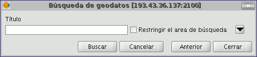
Click on the button and the window will drop down to show more fields which will allow you to carry out an advanced search. The fields you can search in are set by the server. This means that some of the search fields in this form may have no effect in some servers.
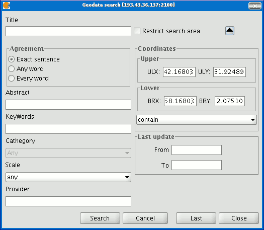
If you change the view zoom, the new coordinates will be reflected in this form. If you wish to restrict the search area enable the corresponding check box. Then click on “Search” and wait for the search to be carried out.
Viewing the results
If the search has been successful, a new window containing the search results will open.
Use the “Previous” and “Next” buttons to see each of the results obtained.
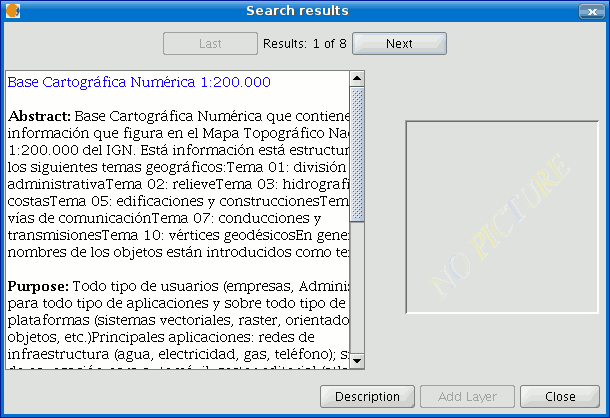
The left-hand side of the window shows information about the metadata obtained. If you wish to see all the information, click on the "Description" button.
You will also be able to see a miniature image at all times, metadata permitting.
If the metadata has any geodata associated to it, the “Add layer” button will be enabled.
gvSIG can currently recognise different types of associated resources, such as WMS, WCS, Postgis tables and web pages.
If you click on this button, a new window will be opened and will show all the resources the application has been able to find.
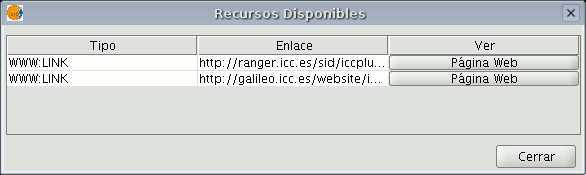
If you click on a WMS, WCS or Postgis type resource, the new layer will automatically be loaded in gvSIG. If the resource is a web page, for example, the operating system’s default browser.
Gazetteer
Introduction
A gazetteer is a data set in which a link is established between a toponym and its geographic coordinates.
gvSIG has a catalogue client which allows you to search by toponyms and centre the view on a specific point.
Connecting to a server
Create a view first and open it. The following button will appear automatically in the gvSIG tool bar.

Click on the button. A wizard opens to help you to carry out a search. The parameters to be input are:
- The server address.
- The server protocol, which in the case of the gazetteer can be:
- WFS-G: Toponym search protocol defined by the OGC.
- WFS: Although this protocol was created with a different purpose in mind, it can be used for a toponym search, as long as it has a text attribute in one of the tables. This protocol also allows you to carry out a “Feature” search in any other field, but not necessarily a text attribute.
- ADL: Protocol specified by the Alexandria Digital Library.
- IDEC/SOAP: Protocol that uses the Catalonian Cartographic Institute (ICC) gazetteer web service.
When you have input all the parameters, click on the "Connect" button and wait until the server is found and accepts the specified protocol. If it is accepted, a new window will appear to start the search. If not, an error message will appear.
Searching
To carry out a search, you will need to fill in the criteria that appear in the following form. You can see the simplified form or carry out an advanced search by clicking on the button in the top right hand corner. This drops down the window.
If you change the view zoom, the new coordinates will be reflected in this form. If you wish to restrict the search area activate the corresponding check box. There are also three options in the “Aspect set up” box which you can use to set up the search view:
Zoom to search: This puts the toponym found in the centre of the gvSIG view.
Delete old searches: This deletes all the texts found in the previous searches from the view.
Draw result: This draws a point and a text label in the place the resulting toponym has been found.
When you have filled in all the fields in the form, click on “Search” and wait for the search to be carried out.
Viewing the results
A new window containing the search results will open. Use the “Previous” and “Next” buttons to move through the different pages of results.
Finally, select the toponym required and click on “Localise”. The gvSIG view will centre on the point the toponym is located in.
Hiperenlace avanzado
The Advanced Hyperlink tool in this version of gvSIG significantly extends the functionality of the hyperlink tool found in version 1.1.
The tool is accessible either from the Layer menu (Layer > Advanced Hyperlink) or by clicking the icon on the toolbar.
Accessing the Hyperlink tool
Hyperlinks are configured at the layer level, which means that they can be enabled or disabled per layer. To set the hyperlink for a layer, double-click on the layer name in the TOC to open the Layer Properties and select the Hyperlink tab.
The hyperlink configuration screen looks like this:
Hyperlink Configuration
Remember that the layer's attribute table must be correctly prepared for the hyperlinks to work. To do this, edit the relevant record and insert the path to the hyperlinked file, leaving out the extension.
After the hyperlinks have been setup and enabled, select the Advanced Hyperlink tool and find the item in the View that corresponds to the record associated with the link. Click on the item and a window will open displaying the linked file.
Actions
The Advanced Hyperlink tool provides the following actions:
- Link to text and HTML files: the tool will open a window in gvSIG and load the linked text or HTML document into it.
- Link to image files: the tool will open a window in gvSIG and load the linked image into it.
- Link to PDF files: the tool will open a window in gvSIG and load the linked PDF document into it.
- Load raster layer: the tool loads the raster layer into the active View.
- Load vector layer: the tool loads the vector layer into the active View.
- Link to SVG files: the tool will open a window in gvSIG and load the linked SVG file into it.
NOTE 1: When editing the hyperlink fields in the attribute table, if a path longer than the maximum field length is entered, the path will be truncated (without warning) to the maximum field length. By default, fields are created with a maximum length of 50 characters. Fields should be defined to handle long paths when necessary, otherwise only very short paths can be stored.
For example: if we enter
C:/Documents and Settings/My documents/images/villafafila.jpg
and the maximum field length is 50 characters, the path will be truncated to:
C:/Documents and Settings/My documents/images/vill
which is not what is wanted.
NOTE 2: Please note that if the path you enter contains an image or file extension that is registered in the registry, you should not also enter it when configuring the hyperlink properties as this would be duplicating the information.
Navigation tools
Navigating around / Exploring the view
Introduction
There are several tools you can use to navigate around the map. These are basically zooms and panning.
Zooms and panning
You can activate these tools by clicking on the "View” menu and then on “Navigation".
or by using the button bar which is quicker. Zoom in: Enlarges a particular area of the view.

Zoom out: Reduces a particular area of the view.

Previous zoom: Goes back to the previous zoom used.

Full extent: Full zoom of the total area included in all the layers of the view.

Panning: This allows you to change the view zoom by dragging the viewing field all over the view with the mouse. Click and hold down the left button of the mouse then move the mouse in the direction you require.

Zoom to selection: Full zoom of the total area of all the selected elements.

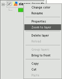
Zoom to layer: To zoom to the layer, right click on the selected layer in the ToC, or click on the “Zoom to layer” option in the contextual menu.
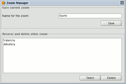
Zoom manager
You can access the “Zoom manager” from the tool bar by clicking on the following button:

or from the “View” menu, then “Navigation” and “Zoom manager”.
By clicking on the “Zoom manager” you can save a zoom so that you can go back to it at a later stage.
This tool can be used to name the current zoom of the view with the text bar which appears in the window.
Click on “Save” and the zoom currently in the view will automatically be added to the “Zoom manager” text box.
You can create and save as many zooms as you wish. Use the "Select” and “Delete” buttons to manage your working areas.
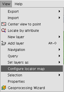
Configuring the locator map
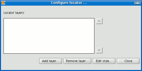
The locator is a general map which is displayed in the bottom left hand corner of the view's window. It is used to show the working area (main window zoom). Click on “View” in the menu bar and select “Configure locator map”.
A window appears in which we can add layers (we can add the same types of layers as in the view) which will make up part of the locator map. This window can also be used to remove layers or edit the layers’ legends.
When you click on the “Add layer” button, the following window appears
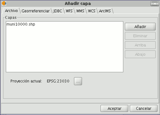
This new function allows the layer loaded in the locator map to be reprojected. To do this, click on the button next to “Current projection when you have selected the layer you wish to load in the locator map.
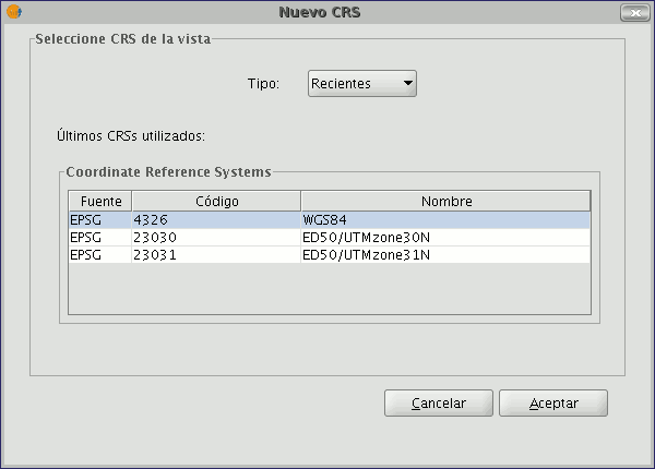
In the following window, select the reference system you wish the layer to have in the locator map and click on “Finish” for the changes to take effect.
Centring the view on a point
This tool allows you to locate a point in the view by its coordinates and to centre the view on this point.

You can also access the tool by going to the “View” menu then to “Centre view on a point”.
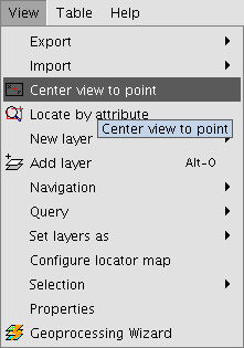
When you have accessed the tool, a dialogue box will appear in which you can input the required coordinates and select the point colour.
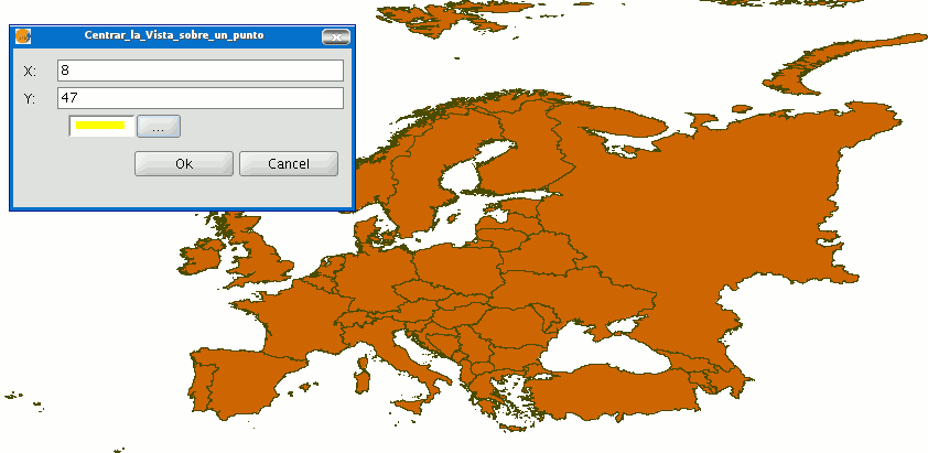
When you click on the "Ok" button, the view centres on this point and the information window that corresponds to this point appears.
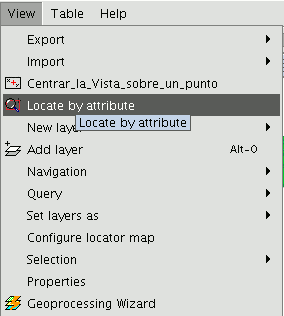
Locate by attribute
This tool allows you to zoom in on areas of a layer by specifying the value of a particular attribute. You can access this tool by clicking on the button

or by going to the “View” menu then to “Locate by attribute”.
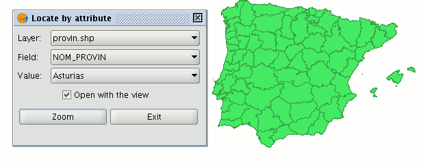
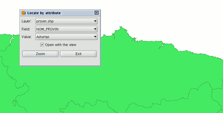
When the tool is selected, the following window appears
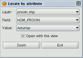
You will find all the layers loaded in the ToC in the “Layer” pull down menu. The fields associated with the chosen layer are included in the “Field” pull down menu.
The data included in the selected field appears in the "Value" pull down menu.
If you mark the “Open with the view” check box and decide to close the view, the “Locate by attribute” window will appear the next time you open the view.
When you have made the selection, click on the "Zoom" button and the chosen area will be shown in the view.
Load data
Geographical data
Introduction
Firstly, open a “View” document in gvSIG.
You can access this option by going to the "View" menu and then to "Add layer" or by using the “Control + O” key combination
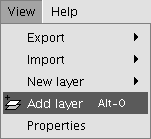
or by clicking on the "Add layer" button in the tool bar.

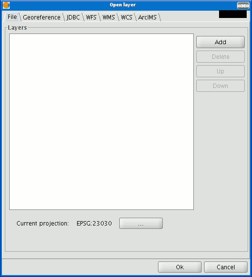
A window appears in which you can select and configure the layer's data source by its type:
Vectorial
Adding a layer from a disk file
Click on the "Add" button
The "Add” dialogue window allows you to move around the file system to select the layer to be loaded. Remember that only the files of the type selected will be shown. To indicate the type of file to be loaded, select a file from the “Files of type” pull down menu.
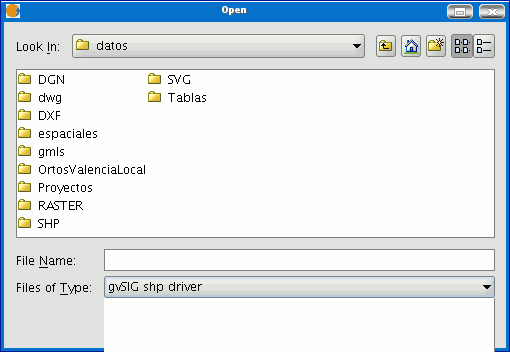
If several layers are loaded at the same time, the order in which the themes will be added to the view can be specified with the "Up" and "Down" buttons in the “Add layer" dialogue.
Adding a layer using the WFS protocol
The Web Feature Service (WFS) is one of the OGC standards (http://www.opengeospatial.org) which is included in the list of standards (of this type) that gvSIG supports.
WFS is a communication protocol via which gvSIG retrieves a vector layer in GML format from a supporting server. gvSIG retrieves the geometries and attributes associated to each "Feature” and interprets the contents of the file.
Go to the “Add layer” and then select the WFS tab.
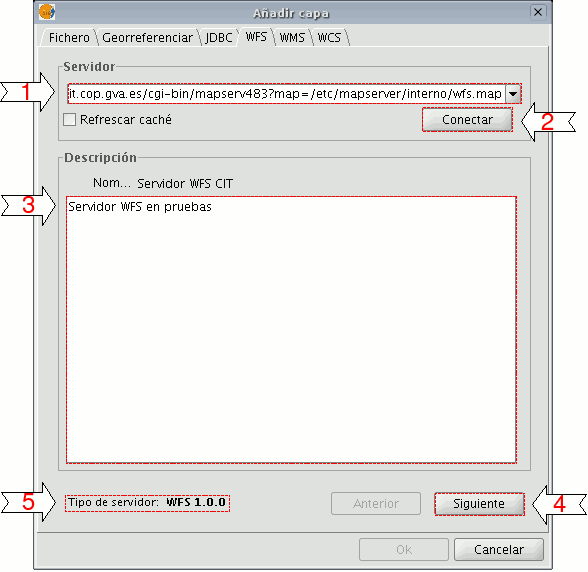
1. The pull-down menu shows a list of WFS servers (you can add a different server if you don’t find the one you want).
2. Click on “Connect”. gvSIG connects to the server.
3. and 4. When the connection is made, a welcome message from the server appears, if this has been configured. If no welcome message appears, you can check whether you have successfully connected to the server if the “Next” button is enabled.
5. The WFS version number that the server you have connected to is using is shown at the bottom of the box.
N.B. You can select the “Refresh cache” option which will search for information from the server in the local host. This will only work if the same server was used on a previous occasion.
Click on “Next” to start configuring the new WFS layer.
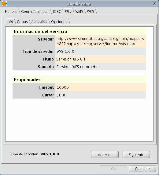
When you have accessed the service, a new group of tabs appears. The first tab (“Information”) shows all the information about the server and about the request that is to be sent. This information is updated as more layers are selected.
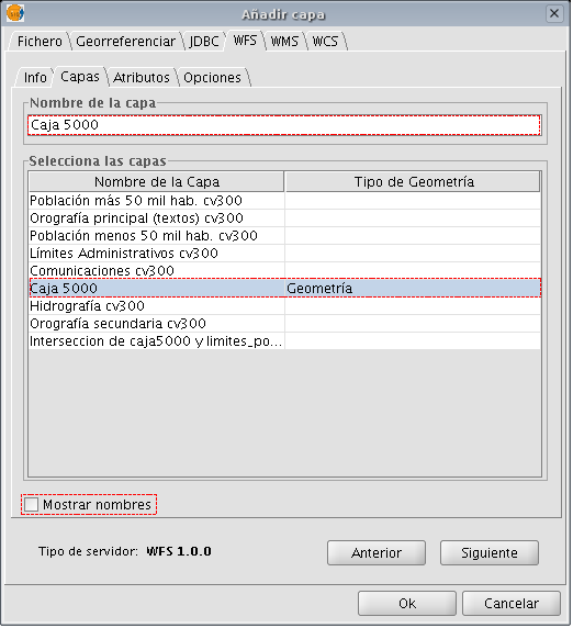
The “Layers” tab can be used to select the layer you wish to load. A two-column table appears in which the layer name and the geometry type are shown. As the geometry type is obtained by clicking on the layer (it needs to be obtained from the server), this column is completely blank at the start.
The “Show layer names” option shows the name of the layer as it is recognised by the server and not by its description, which is what appears in the table by default.
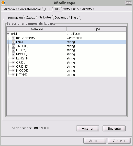
The “Attributes” tab allows the fields (or attributes) of the selected layer to be selected. When the layer is loaded, only the fields that have been selected are retrieved.
To select the attributes, enable the check box which appears to their left.
The "Options” tab shows information about user authentication and the connection. The “User” and “Password” fields are used in the WFS-T to be able to identify a user in the server so that writing operations can be carried out (not yet implemented).
The connection parameters are:
Number of features in the buffer, i.e. the maximum number of elements that can be downloaded.
Timeout. This is the length of time beyond which the connection is rejected as it is considered to be incorrect. If these parameters are very low, a correct request may not obtain a response.
The Spatial Reference System (SRS) is another important parameter. Although this cannot currently be changed, it is hoped that this will be possible in the future. In any case, gvSIG reprojects the loaded layer to the spatial system in the view.
You can use this tab to apply filters to your WFS layers. Click on the “Filters” tab in the window.
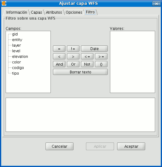
The “Fields” text box shows the layer’s attributes which can be used as a filter. Click on the selected field to see its values.
When the layer is loaded for the first time, the values in the column cannot be selected. However, if you have a filter sentence for the layer you can apply it in the filter text area and the filtered layer will be loaded directly.
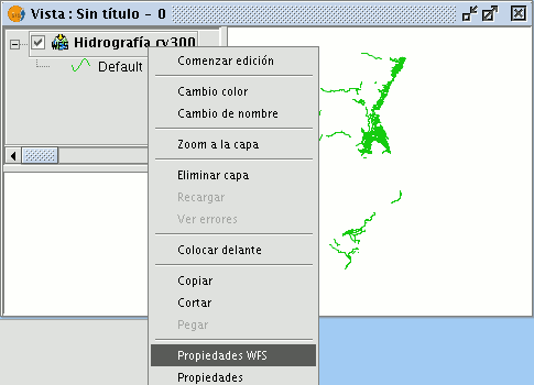
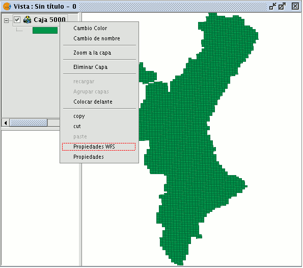
If you do not have a filter sentence, load the WFS layer into the ToC, then right click on the mouse and select the “WFS properties” option from the contextual menu.
To create the filter for the WFS layer, double click on the field you wish to use as a filter and it will appear in the bottom text area. Then click on the operator you wish to apply and finally select the value in the “Values” text area by double clicking on it.
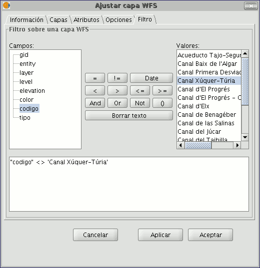
When you have created the required filter, click on “Ok” and it will be applied to the WFS layer.
When all the parameters have been configured, click on “Ok”. The layer will be loaded into a gvSIG view.
By right clicking on the layer, its contextual menu appears. If the “WFS Properties” option is selected, an option display opens (similar to the “Add layer” display). This can be used to select new attributes and other layers and change the layer’s properties.
In gvSIG 1.9 a new 'Area' tab was added which allows the user to filter the requested WFS layer geometries according to a bounding box. The user enters the coordinates of the required display area so as to optimize access to the data layers and to save time when viewing them.
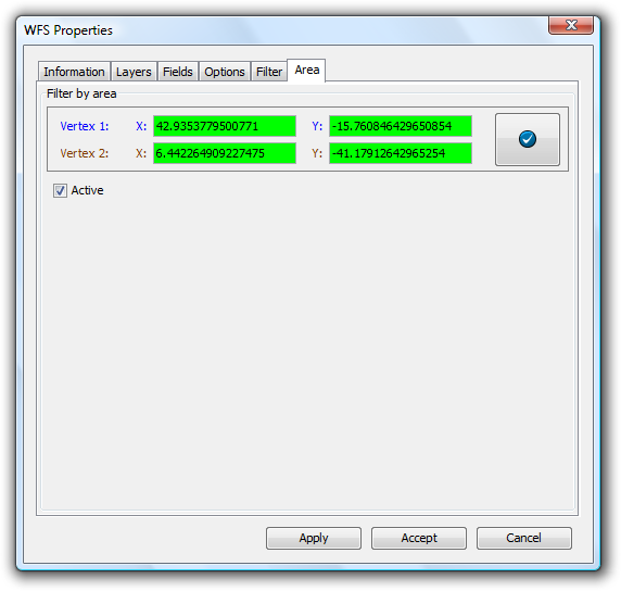
Loading a WFS layer - The Area tab
Adding a layer using the ArcIMS vectorial
In the proprietary software environment, ArcIMS (developed by Environmental Sciences Research Systems, ESRI) is probably the most widespread/popular widely used (Internet) cartographic server on the Internet thanks to the number of clients it supports (HTML, Java, ActiveX controls, ColdFusion...) and to its integration with other ESRI products. ArcIMS is currently one of the most important remote cartographic information providers. Although the protocol it uses does not comply with the Open Geospatial Consortium (because it was created long beforehand), the gvSIG team believes that offering support for ArcIMS is important.
The extension can access image services offered by an ArcIMS server. This means that, just like a WMS server, gvSIG can request a series of layers from a remote server and receive a view rendered by the server containing the requested layers in a specific coordinate system (reprojecting if necessary) and in specific dimensions. In addition to displaying geographic information, the extension allows you to request information about the layers for a particular point via the gvSIG standard information button.
ArcIMS is slightly different in its philosophy from WMS. In WMS, the request is normally made by independent layers whilst in ArcIMS the request is global.
The steps required to request a layer from an ArcIMS server and to request information for a particular point are listed below.
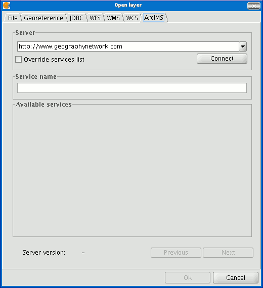
Our example uses the ESRI ArcIMS server. Its URL is http://www.geographynetwork.com. This is the address a web browser requires to access the HTML visual display unit.
Before loading a layer from this server, the datum WGS84 in geodesic coordinates (code 4326) has to be set up previously as the view’s spatial system.
If the extension is loaded correctly, a new ArcIMS data source will appear in the “Add layer” dialogue box.
Adding a new layer to the view
If the server has a standard configuration, simply indicate its address. gvSIG will try to find the servlet’s full address.1 If the servlet has a different path, you will have to write it into the dialogue box.
When the connection has successfully been made, the server version, its compilation number and a list of image and geometry services available are shown.
The service can be selected from the list or can be written in directly.
Finally, if the “Override service list” check box is enabled, gvSIG will delete any catalogue that has already been downloaded and will request them again from the server.
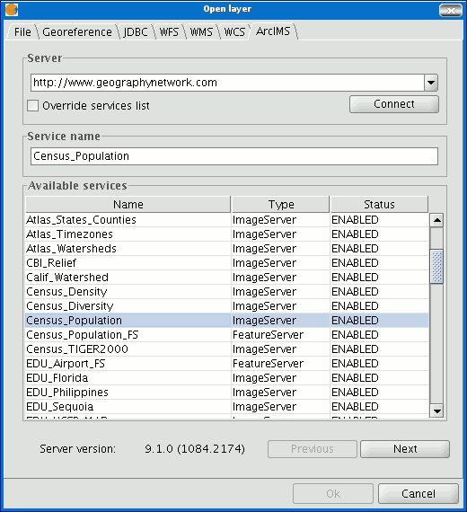
List of services available
The next step is to select the ImageServer type service required by double clicking or selecting it and clicking on "Next". The dialogue box changes and an interface with two tabs appears (fig. 3). The first tab shows the metainformation given by the server about the service’s geographic limits, the acronym of the language it has been written in, units of measurement, etc. It is a good idea to find out if a coordinate system has been defined in the service (using EPSG codes) as this can directly influence the requests made to the server, as Figure 3 shows.
N.B. If no coordinate system has been defined in the service, the extension will assume that it is the same coordinate system as the one we have defined for the view.
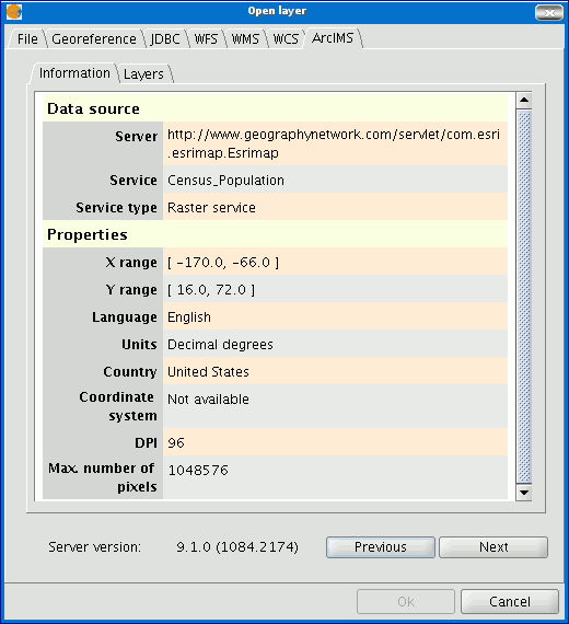
Figure 3: Metadata from the ArcIMS server
We can continue by clicking on "Next" or return to the previous dialogue by clicking on "Change service”.
The last dialogue box is the layer selection. We can define a name for the gvSIG layer or leave the default value (the service name) in this window. A box appears below with a list of the service layers in tree form. When the mouse is moved over the layers, information about these layers appears: extension, scale ranges, type of layer (raster or vector image) and if it is visible by default in the service (fig. 4).
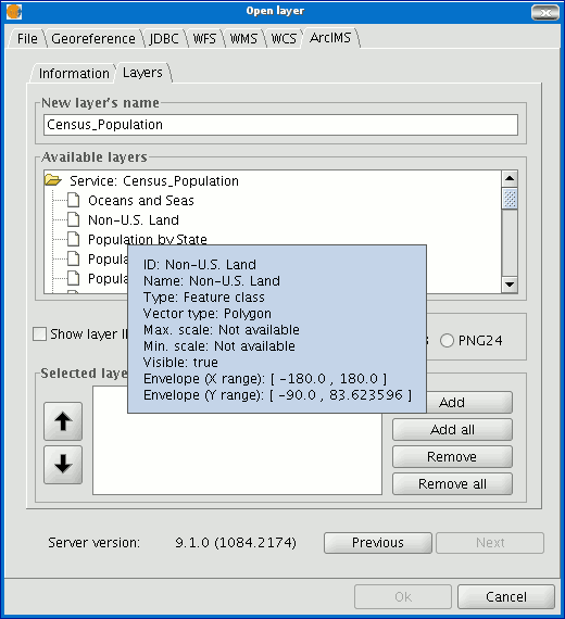
Figure 4: Metadata from a service layer
We can view each layer’s ID via the “Show layer ID” check box. This check box is useful when there are layers whose descriptor is repeated. Therefore, the only way to distinguish between them is via an ID, which will always be unique. A combo box is also available to select the image format we wish to use to download the images. We can choose JPG format if our service works with raster images or one of the other remaining formats if we want the service to have a transparent background.
N.B. The transparency in 24-bit PNG images is not correctly displayed in gvSIG 0.6. This type of files will be supported in gvSIG 1.0.
The box with the layers selected for the service appears below. If you wish, you can add just some of the service layers and also reorganise them. This makes the service view totally personalised.
N.B. The configuration cannot be accepted until a layer has been added.
N.B. Multiple selections of service layers can be made by using the Control and CAPS keys.
When the “Ok” button in the dialogue box is pressed, a new layer appears in the view (fig. 5). If no layer has been added previously, the extension of the ArcIMS layer is shown, as per the standard gvSIG procedure.
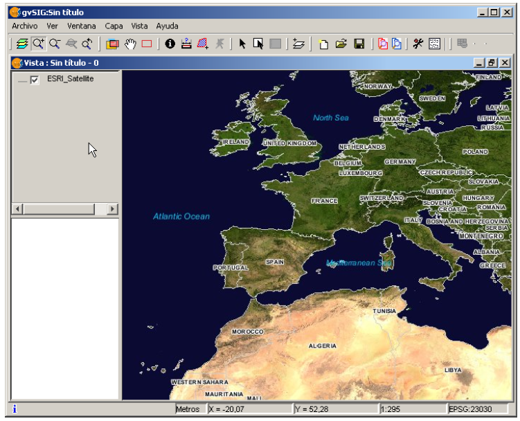
Figure 5: ArcIMS layer added to the gvSIG view.
It must be remembered that when the layer extension is shown, the layers that make up the chosen configuration may not appear and a blank or transparent image appears instead. If this occurs, use the scale control dialogue box (V. Information about scale limits section).
An ArcIMS server does not define the spatial reference systems it supports as opposed to the WMS specification. This means that a priori we do not have a list of EPSG codes that the map server can reproject. In short, ArcIMS can reproject to any coordinate system and leaves the responsibility of how the projections are used to the client.
Therefore, if our gvSIG view is defined in ED50 UTM zone 30 (EPSG:23030) and we request a global coverage service (stored for example in the geographic coordinates WGS84, which correspond to code 4326) the server will not be able to reproject the data correctly because we are using global coverage for a projection of a specific area of the Earth.
However, the procedure can be carried out in reverse. If we have a view in geographic coordinates (and thus global coverage), services defined in any coordinate system can be requested because the server will be able to transform the coordinates correctly.
In short, requests to the ArcIMS server must be made in the view's coordinate system and they cannot be requested in another coordinated system.
Moreover, as we mentioned above, if an ArcIMS server does not offer information about the coordinate system its data is in, the user will be responsible for setting up the correct coordinate system in the gvSIG view. Thus, if a user with a view in UTM adds a layer which is in geographic coordinates (even though the server does not show it), the service will be added correctly but will take the view to the geographic coordinates domain (in sexagesimal degrees).
An additional effect is that if the view uses different units of measurement from the server, the scale will not be shown correctly.
The layers requested from the server can be modified via a dialogue box, which can be accessed from the layer’s contextual menu (fig. 6) just like the WMS layers. This dialogue box is similar to the box used to load the layer, apart from the fact that the service cannot be changed.
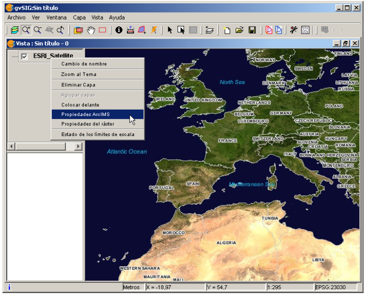
Figure 6: Properties of the ArcIMS layer
The extension allows us to consult the layers' scale limits which make up the requested service via a dialogue box which can be maintained in the view during the session (fig. 7). This window shows the layers on the vertical axis and the different scale denominators on the horizontal axis via a logarithmic scale. This box is small on screen but can be enlarged to improve the difference between the scales.
The vector layers, raster layers and the layers that can be seen on the current scale (marked with a vertical line) in a darker colour and the layers we cannot see above or below the current scale are differentiated by different coloured bars (described in the window legend).
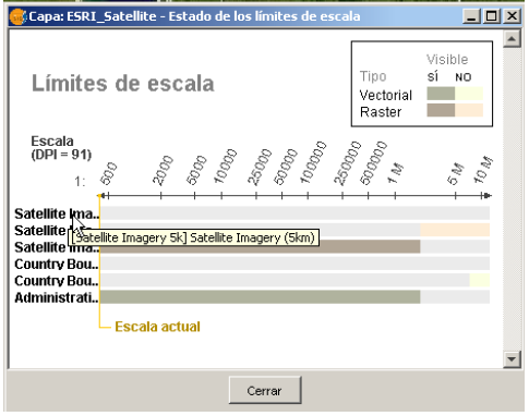
Figure 7: Scale limits status
Attribute information requests about the elements for a particular point is one of gvSIG’s standard tools. Its functionality is also supported by the extension.
The WMS specification allows information about several layers to be requested from the server in one single query. This is different in ArcIMS. We need to make one server request per layer required.
This means that no requests for unloaded layers or unseen layers that are not visible on the current scale or layers whose extension is outside the view will be made. Even if all these layers are filtered, the information request usually takes longer than is desirable because of this intrinsic feature of ArcIMS.
When all the request responses have been recovered, the standard gvSIG attribute information dialogue appears with each of the layers (LAYER) which return information as a tree. If we click on a layer, its name and ID appear on the right (fig. 8).
Under this node, if we are talking about a vector layer, all the records or geometric elements the server has responded to appear, and give each one their corresponding attributes (FIELDS).
If it is a raster layer, such as an orthoimage or a digital terrain model, it returns the values for each of the bands (BAND) in the requested pixel colour, instead of records.
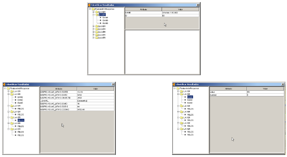
Figure 8: Displaying attribute information
The extension allows access to both ArcIMS image services and geometry services (Feature Services). This means that a server can be connected to and geometric entities (points, lines and polygons) and their attributes obtained. This is not dissimilar to WFS service access.
However, the variety of existing geometry services is much lower than the variety in the image server. There are two main reasons for this. On one hand, providing the public with vector cartography implies security problems because many bodies only want to offer the general public views and images. The vector data becomes either an internal product or must be paid for. On the other hand, this type of services generate much more traffic on the network and in the case of basic information servers could become a problem.
Loading a geometry layer is practically the same procedure as loading the image server as mentioned above (Accessing the service section and the following sections). In this case, the number of layers to be selected must be taken into account. If we wish to download all the layers offered by the service the response time will be very high.
The only difference between loading an image layer is that in this case we can choose whether we wish the layers to be downloaded as a group via a check box. This is useful for processing the vector layers as one layer when it needs to be moved and activated in the table of contents.
Unlike the image service, in which all the service’s layers appear as one unique layer in the gvSIG view, in this case each layer is downloaded separately and appears in the view grouped under the name defined in the connection dialogue.
Cartography symbols are configured in the server in one AXL extension file for both geometry and image services. We can divide symbol definition into two parts. On one hand, we can talk about the definition of the symbols themselves, i.e. how a geometric element, such as a line or polygon, should be presented. On the other hand, we can talk about the distribution of these symbols according to the cartographic display scale or to a specific theme attribute.
In ArcIMS terminology symbols are different from legends (SYMBOLS and RENDERERS).
There are various types of symbols: raster fill symbols, gradient fill symbols, simple line symbol, etc. The extension adapts the majority of the symbols generated by ArcIMS. Table 1 shows the ArcIMS symbols and indicates whether they are supported by gvSIG.
| Label | Description | Supported |
|---|---|---|
| CALLOUTMARKERSYMBOL | Balloon-type label | NO |
| CHARTSYMBOL | Pie chart symbol | NO |
| GRADIENTFILLSYMBOL | Fill in with gradient | NO |
| RASTERFILLSYMBOL | Fill with raster pattern | YES |
| RASTERMARKERSYMBOL | Point symbol using pictogram | YES |
| RASTERSHIELDSYMBOL | Customised point symbol for US roads | NO |
| SIMPLELINESYMBOL | Simple line | YES |
| SIMPLEMARKERSYMBOL | Point | YES |
| SIMPLEPOLYGONSYMBOL | Polygon | YES |
| SHIELDSYMBOL | Point symbol for US roads | NO |
| TEXTMARKERSYMBOL | Static text symbol | NO |
| TEXTSYMBOL | Static text symbol | YES |
| TRUETYPEMARKERSYMBOL | Symbol using TrueType font character | NO |
Table 1: ArcXML symbol definition labels
In general, the most common symbols have been successfully “transferred”. Some of the symbols cannot be obtained directly from gvSIG (at least in the current version), such as the raster fill symbol or they need to be “adjusted” such as the different types of lines. This means that a raster fill symbol is not a symbol that can be defined by the gvSIG user interface, but it can be defined by programming.
gvSIG supports the most common types of legends: unique value and range and value themes as well as the scale-range control over the whole layer. ArcIMS goes much further in its configuration. It can generate much more complicated legends in which symbols can be grouped together, scale-range controls can be established for labels and symbols and different labelling based on an attribute can be shown (as though it were a value theme for labelling).
This group of legends can generate very complex symbols for a layer in the end. The current implementation status of the gvSIG symbols needs to be simplified to reach a compromise to recover the symbols that best represent the layer as a whole.
| Label | Description |
|---|---|
| GROUPRENDERER | Legend which groups others together |
| SCALEDEPENDENTRENDERER | Scale dependent legend |
| SIMPLELABELRENDERER | Labelling layer legend |
| SIMPLERENDERER | Unique value layer legend |
| VALUEMAPRENDERER | Value and range themes |
| VALUEMAPLABELRENDERER | Labelling themes |
Table 2: ArcXML legend definition labels
When a GROUPRENDERER is found, the symbol ArcIMS draws first is always chosen. Thus, in the case of the typical motorway symbol for which a thick red line is drawn and a thinner yellow line is drawn over it, gvSIG will only show the red line with its specific thickness.
If a scale dependent legend is discovered during a symbol analysis, this is always chosen. If more than one is discovered, the one with the greatest detail is chosen. For example, in ArcIMS we can have a layer with simple road symbols (only main roads are drawn) on a 1:250000 scale and based on this a different theme is shown with all types of roads (paths, tracks, roads, etc.). In this case, gvSIG will show this last theme as it is the most detailed.
If a labelling legend is discovered during a symbol analysis, it will be saved in a different place and will be assigned to the selected definitive legend. In the case of the VALUEMAPLABELRENDERER label, only the legend of the first processed value will be obtained as a label symbol. The rest will be rejected.
In short, it is obvious that the failure to adapt the legends for gvSIG is a simplification process in which different legend and symbol definitions must be rejected to obtain a legend which is similar to the original as far as possible. It is to be expected that the gvSIG symbol definition will improve considerably so that it can support a larger group of cases in the future.
Working with the layer is similar to any other vector layer, as long as we remember that access times may be relatively high. The layer attribute table can be consulted, in which case the records will be downloaded successively as we display them.
If we wish to change the table symbols to show a unique value or range theme we must wait as gvSIG requests the complete table for these operations. On the other hand, the downloading of attributes is only carried out once per layer and session and therefore, this wait only occurs in the first operation.
In general, if our ArcIMS server is in an Intranet, it will be relatively fast to handle, but if we wish to access remote services we may be faced with considerable response times.
The main feature to bear in mind when working with an ArcIMS vector layer is that the geometries available at any given time are only the ones displayed. This is because we can connect to huge layers but only the visible geometries are downloaded. As far as gvSIG is concerned, the geometries shown on the screen are the only ones available and thus, if we export the view to a shapefile for example, are only a part of the layer.
Finally, we need to remember that to speed up the geometry downloads they are simplified to the viewing scale in use at any given time. This drastically reduces the amount of information downloaded as only the geometries that can actually be "drawn" are displayed in the view.
Loading a geometry layer is practically the same procedure as loading the image server as mentioned above (Accessing the service section and the following sections). In this case, the number of layers to be selected must be taken into account. If we wish to download all the layers offered by the service the response time will be very high.
Unlike the image service, in which all the service’s layers appear as one unique layer in the gvSIG view, in this case each layer is downloaded separately and appear in the view grouped under the name defined in the connection dialogue.
After a few seconds the layers appear individually but are grouped under a layer with the name we have defined for it.
The layer symbols are established at random. A pending feature is to recover the service symbols and configure them by default so that gvSIG can display the cartography as similarly as possible to how it was established by the service administrator.
geoDB Extension (database manager)
This extension allows users easy, standardised access to geographic databases from different providers. At present, gvSIG supports the following database management systems:
| Data bases | Read | Write |
|---|---|---|
| PostgreSQL/PostGIS | Yes | Yes |
| MySQL | Yes | No |
| HSQLDB | Yes | No |
| Oracle (SDO Geometry) | Yes | Yes |
gvSIG stores the different connections made during the various sessions. Thus, users do not need to input the parameters of every server they connect to. Likewise, if a project file is opened which has a database connection, the user will only be required to enter the password.
The extension has two user interfaces, one to manage the data sources and another to add the layers to the view.
Select the menu See – Spatial database connection manager (figure 1) to open the dialogue box which allows you to add, remove, connect and disconnect the connections to the different types of databases containing geographic information. If you have already used this manager in an earlier gvSIG session, the previous connections will appear (figure 2). If not, the dialogue box will be empty.
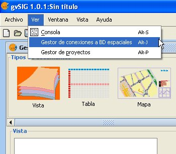
Figure 1. Access to the geoDB connection manager
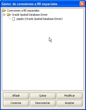
Figure 2. The connection manager
Click on Add to introduce the parameters of a new connection (figure 3). NB: From gvSIG version 1.1 onwards, it should be noted that the name of the database must be written correctly and that it is case sensitive. If you wish to open a project saved in a version prior to gvSIG 1.1 which includes layers belonging to a database whose connections have not taken this factor into consideration, the data must be recovered by reconnecting to the original data base. You can either connect there and then or remain offline. Open connections appear with a link and with “[C]” before their name (figure 4). If you wish to open a connection, select it and click on Connect. You will be asked to enter the password (figure 5) and the connection will then be made.
Figure 3. Adding a new connection
Figure 4. The connection has been made
Figure 5. Password request
In the Project Manager, create a new view and open it using the New and Open buttons. Use the Add layer icon to add a layer to the view. Go to the GeoDB tab in the dialogue box to add a new layer of this type (figure 6). You must choose a connection (if you select one which is disconnected, you will then be asked to enter the password), select one or more tables and the attributes you wish to download from each layer and, optionally, set an alphanumeric restriction and an area of interest. You can give each layer a different name to that of the table. Click on Ok to view the table’s geometries in the view. This window also allows you to specify a new connection if the database is not registered in the data source catalogue. Any alphanumeric restriction must be introduced by means of a valid SQL expression which is attached as a WHERE clause to each call to the database. Given that the table may take several seconds to load, a small icon appears next to the name of the table indicating that this process is underway. When the table has been loaded, the small blue icon disappears and the gvSIG view is automatically refreshed to allow the geometries to be viewed.
Figure 6. Adding a geoDB layer
Figure 7. Views with geometries from a geographic database
Figure 8. Mini icon showing layers are loading
This function allows new tables to be created in the spatial database from any vectorial source in gvSIG. These tables can be created as follows:
- Create a vectorial layer of any type, for instance by opening an SHP file using the Add layer button (figure 9).
- Select the layer by clicking on its name in the left-hand side of the screen (figure 10).
- In the Layer – Export to menu, select the type of database you wish to export the layer to. The example shows an Oracle database (figure 11).
- You will then be asked to introduce the name of the table which will be created in the database (Oracle) and whether or not you wish to include the newly-created layer in the current view.
If all goes well, the new vectorial geoDB layer will appear in the view and you will be able to work with it in the usual way.
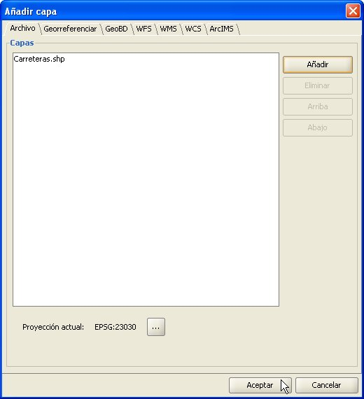
Figure 9. Adding a vectorial layer

Figure 10. Selecting the layer to export
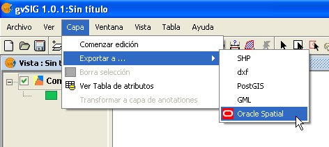
Figure 11. Exporting to Oracle Spatial
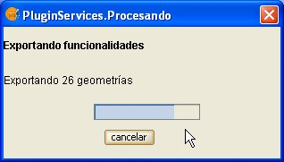
Figure 12. Export progress bar
These notes supplement the documentation for the geoDB extension with regard to the driver for Oracle Spatial.
This driver allows access to any table from an installation of both Oracle Spatial and Oracle Locator (in both cases from version 9i onwards) which has a column that stores SDO-type geometries.
The driver only lists tables which have their geographic metadata in the USER_SDO_GEOM_METADATA view.
Given that each table’s metadata is available, the interface makes use of that data and automatically presents the column (or columns) of geometries. Likewise, ROWID, which is a unique descriptor for each row used internally by Oracle, is used and this ensures that identification is correct.
Two and three-dimensional data of the following types are supported:
- Point and multipoint
- Line and multiline
- Polygon and multipolygon
- Collection
At present, layers in LRS format (Linear Referencing System) are not supported.
Oracle has its own system for cataloguing coordinate and reference systems. Miguel Ángel Manso, on behalf of the Polytechnic University of Madrid, has provided a list of equivalent values for the Oracle system and the EPSG system and this is included in the driver as a DBF file.
Conversions from one coordinate system to another are carried out by gvSIG since its performance has proved to be superior.
The driver constantly performs geometric requests (in other words constantly calculates which geometries intersect with the current gvSIG view) and it is therefore essential that the database has a spatial index linked to the column in question.
If this index does not exist, an error window appears (figure 1) and the table or view cannot be added to the gvSIG view.
In addition, the driver needs to set a unique identifier for the records of the table or view, and this is not possible for certain types of views. If such a problem occurs, it will be detected by the driver and an error message will also appear (figure 2).
As a result, the view cannot be loaded to gvSIG from the database.
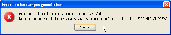
Figure 1. Warning regarding the lack of a spatial index
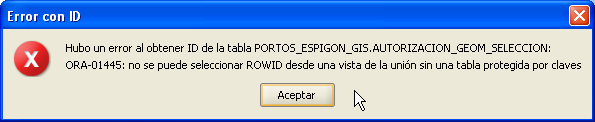
Figure 2. Warning regarding the fact that a ROWID could not be obtained
If you wish to export a layer to an Oracle database, you will also be asked if you wish to include the view’s current coordinate system in the table at the end of the process described in the manual. This may be useful in cases where we do not wish to include such information in the table for reasons of compatibility with other applications or information systems.
To work with two Oracle geometries (the most common case is an intersection), the two geometries must have the same coordinate system. Each geometry has an SRID field which can have the value NULL.
For instance, if we have a table with geometries in EPSG:4326 (Oracle code 8307) and another with geometries in EPSG:4230 (Oracle code 8223), it will not be possible to carry out SQL instructions to perform calculations directly between the geometries of one table and another. However, if these tables’ geometries do not have a coordinate system (i.e. SRID is NULL), then operations can be performed between the geometries of these tables, bearing in mind the errors involved in carrying out intersections between different coordinate systems.
When reading a table whose geometries have a coordinate system set at NULL, it is understood that the user will make sure that the geometries are appropriate for the current view, since no reprojection is possible (this may change with the new gvSIG extension for the advanced use of coordinate systems).
In short, not storing the coordinate system allows for a more flexible use of geometries.
If you have previously used the connection manager in a previous gvSIG session, the connections will have been preserved. Otherwise, it will be empty:
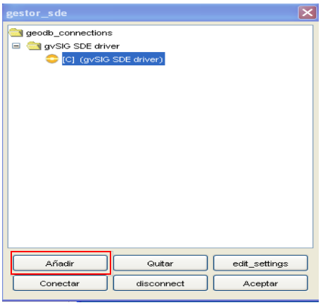
Click "add" and a window that allows you to enter new connection parameters will show up. Fill the data fields and click "OK". Note: In the drop-down selections of “Driver” select the one that corresponds to "gvSIG SDE driver", as shown in the image.
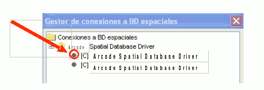
Once the connection is validated, it brings back the "connection manager" with the new database in the list. If in the connection settings window the "connected" box is left checked, the connection will remain open. Open connections are marked "[C]" before its name.
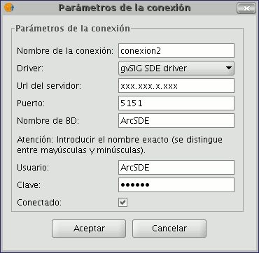
If you want to disconnect the connection click on "disconnect" at the bottom of the manager. The connection will stop at the time, but the parameters will remain recorded for future connections. If you want to open a connection that is already included in the list for having been previously used, you must select it and click "Connect". It will ask for the password again in a window like in the following figure represents and the connection will be open.
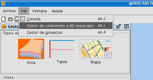
Choose the menu "View / Spatial BD connection manager" to open the dialogue that lets you add, remove, connect and disconnect connections to different types of databases with geographic information:
Once we have established the connection to the server, we can begin to query information from it.
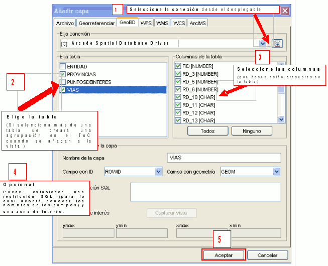
For this we will open a view and press the button "Add layer".

Then select the GeoBD tab.
. In the dropdown list you can select your connection. The button to the right side of the box can take you directly to the connection settings window, in case you want to add a connection in some other time without having to go through the connection manager.
. Once the connection is established you will see a list of the available information that can be added to gvSIG.
. From this window you can query or create filters (SQL restrictions) before adding the information.
. Once you select the information you want, click "OK" and it will upload into the view.
Adding an Event layer
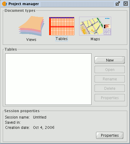
A new layer can be created from a table in gvSIG by using “Add event layer”.
There are two ways to do this: you can add a table to the project or you can work with a table associated with one of the layers in the view in which you are working at a particular time.
Firstly, the table needs to be loaded. To do so, go to the gvSIG “Project manager” and select "Tables" in document types. Then click on "New".
A search dialogue opens to add the table you require. Click on "Add".
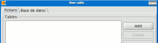
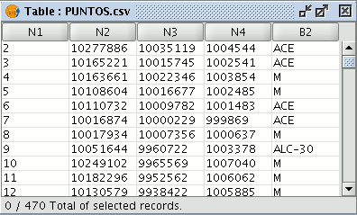
A dialogue box appears in which you can choose two types of data sources: dbf and csv.
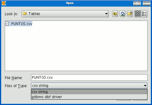
When you have found the table you require, select it and click on “Open”.
gvSIG automatically returns to the "New table" window and adds the table you require to create the event layer in the text box.
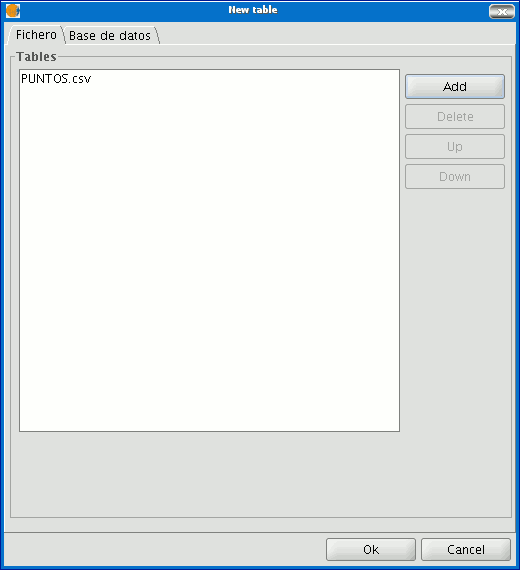
Click on “Ok” to finish the process.
When the table has been added, a view must be active to create its corresponding event layer and load it. If no view is active, you can return to the “Project manager” and add one or create a new blank one. When you have activated this view, go to the “Add event layer” by using the corresponding button in the tool bar:

A window with three pull-down menu bars appears.
We can select the table we need to add the new layer from the first pull-down menu bar.
Then, we can select the table fields which will become the X and Y values.
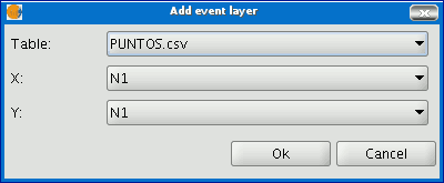
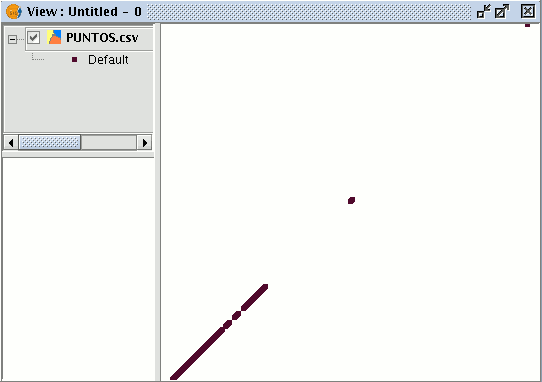
If you click on “Ok”, a new points layer will appear based on the coordinates contained in the initial table.
If you wish to work with a table associated to the layers in the view, you will firstly have to activate the attribute table of this layer. To do so, click on the following button in the tool bar:

If you click on “Add event layer”

you will see that the table has been added.
Coordinate Reference Systems
The jCRS extension intends to bring rigorous CRS handling capacity to gvSIG, as well as the incorporation of the standard CRS operations and repositories like, in this version: EPSG, ESRI, IAU2000 and user-defined CRS.
These added functions provide a solution to the ED50-ETRS89 transition problem, and in accordance with the implementation of the Royal Decree 1071/2007, two solutions are integrated that were achieved by the National Geographic Institute (IGN):
- Through the EPSG, the different official IGN achievements are incorporated following the seven-parameter transformation model.
- Through Proj4, the official IGN grid based transformations with grid files in NTv2 format are incorporated.
Further in this document, the user interface for this extension will be described, using the most common cases.
In the description of these cases, there might be an overlap in CRS selection methods and dialogs. To avoid repetitions, it was considered convenient to explain a dialog in detail the first time that it appears in the manual, and therefore users are advised to read the sections in the correct order.
In this latest version of the jCRS extension, users can define a custom CRS. This functionality is available through the CRS selection dialog, see figure 14.
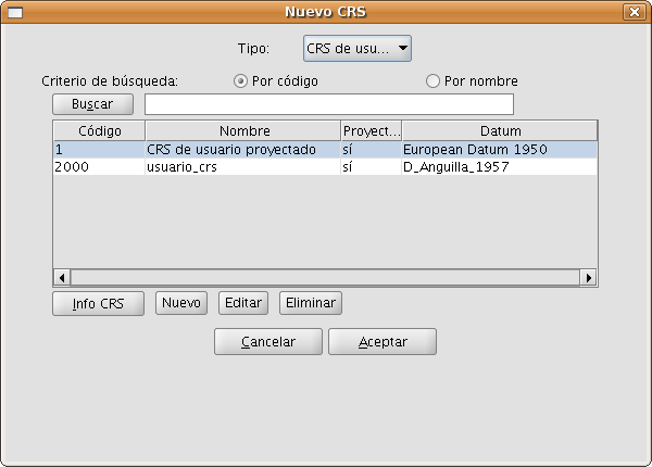
Figure 14: Selection of a user-defined CRS
When selecting User CRS as the type of CRS, you can choose from the following options:
- Choose a custom CRS that was previously defined, by selecting it from the table and click on OK. To facilitate the selection when there are many user-defined CRS, there are two search options to find common CRS: by code and by name.
- To find information on the selected CRS, you can click on the CRS info button, after which a window with the available information will appear.
- To edit the selected CRS, click on the Edit button. A dialog with different tabs will appear which is similar to the dialog in which you can define a new custom CRS. These dialogs will be described later on in this document.
- To delete the selected CRS, click on the Remove button.
- Create a new custom CRS, as described here below.
To create a new custom CRS, click on the New button in the dialog shown in Figure 14, after which the dialog User defined CRS will open (see figure 15) to guide you through the process of creating a custom CRS.
This dialog includes three tabs:
- User CRS, where you can choose between three alternatives to create the CRS:
- From user definitions. With this option, the user will enter all the needed information to create the CRS. When this option is selected, the panels in the Datum and Coordinate system tabs will appear empty so that the user can fill them, although some information (ellipsoid, prime meridian, …) can be taken from other CRS that are included in EPSG.
- From an existing CRS. This option permits the selection of an existing CRS from EPSG, by clicking on the button with three points, load the information in the corresponding panels under the Datum and Coordinate system tabs, and create the custom CRS by modifying this information.
- From a WKT string. This option is similar to the previous one, but here the WKT string is used to load the information of an existing CRS in the corresponding panels of the Datum and Coordinate system tabs.
- Datum, where you can enter the Datum information associated with the CRS.
- Coordinate system, where the information of the coordinate system associated with the CRS is filled.
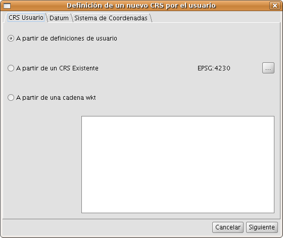
Figure 15: Create a new custom CRS
By clicking the button Next you can move from one tab to the next.
In figure 16, the panel of the Datum tab is shown. In this tab, the following information must be filled:
- Information about the CRS to be defined that will be used in search queries:
- Name. Alphanumeric string to indicate the name of the CRS.
- Code. Integer number to be assigned to the CRS for indexing in the database, this must be a unique number that has not been previously assigned to another custom CRS.
- Information about the datum associated with the CRS:
- Name of the datum. Alphanumeric string to indicate the name of the datum. This can be selected from an existing EPSG CRS by clicking on the button with three points on the right of the text box.
- Ellipsoid. Information on the reference surface of the CRS to be defined. This can be selected from an existing EPSG CRS by clicking on the button with three points on the right of the text box for the ellipsoid name. The information to be filled is:
- Name of the Ellipsoid. Alphanumeric string to indicate the name of the ellipsoid.
- Shape and dimensions of the ellipsoid. You can choose between two options:
- a, inv_f, which refers to the semi-major axis and inverse flattening. To define the semi-major axis correctly it is necessary to enter the value and corresponding unit.
- a, b, which refers to the semi-major and semi-minor axis of the ellipsoid. This option should be chosen when the reference surface is a sphere, in which case the values of both semi-axes are equal and the resulting value of the inverse flattening is infinite. To define correctly both semi-axes of the ellipsoid, the value and corresponding unit must be entered.
- Meridian. Here, the name of the prime meridian that is used for the datum must be filled. You can select the prime meridian from an existing EPSG CRS by clicking on the button with three points on the right of the textbox for the meridian name. The following information must be filled:
- Name of the meridian. Alphanumeric string to indicate the prime meridian.
- Longitude. Geographic longitude relative to Greenwich. The value and corresponding unit must be filled.
The default ellipsoid and meridian for user defined CRS are the GRS80 ellipsoid and Greenwich meridian.
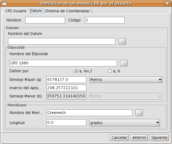
Figure 16: Definition of the datum for the CRS
When the datum parameters are defined, the Coordinate system information associated with the CRS must be filled in the next tab as shown in figure 17.
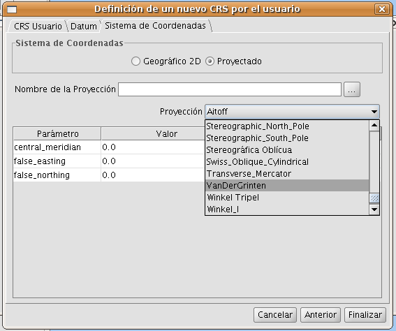
Figure 17: Selection of the coordinate system for the CRS
The following Coordinate system information must be filled:
- Coordinate system: Geographic 2D or Projected.
- In case of a projected coordinate system, the following must be filled:
- Name of the projection. Alphanumeric string to indicate the name of the projection.
- Projection. One of the available options of the drop-down list must be chosen.
- Projection parameters: Value and unit. The list of parameters will change according to the type of cartographic projection.
To edit a custom CRS that was previously defined (see figure 14), select this CRS from the table and click on Edit.
Below in figure 18 the dialog Definition of a new custom CRS is displayed, where the tab User CRS is disabled as well as the CRS code in the Datum tab. The reason why you can not modify the CRS code is that this code is used for the indexation of the user database. The other values for the datum are editable, as well as the values for the Coordinate system tab (see figure 19).
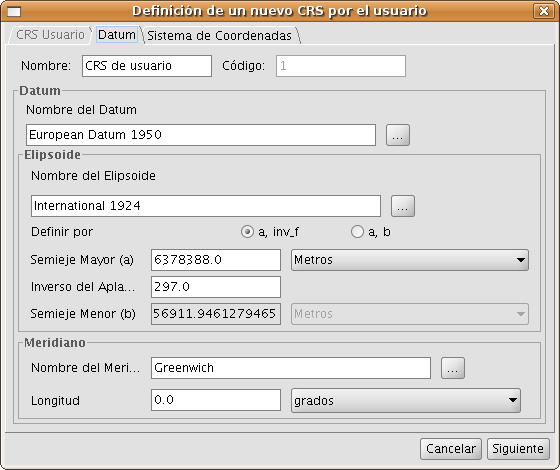
Figure 18: Editing of the datum values
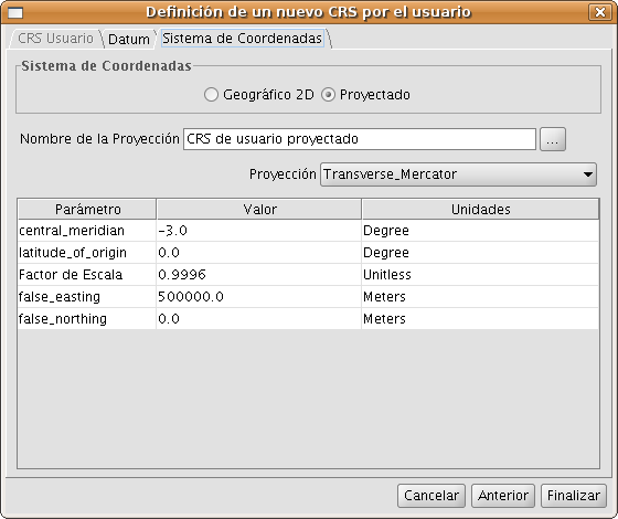
Figure 19: Editing of the coordinate system of the CRS
The selection of the CRS for a layer can be done by adding the layer to a view, and clicking on the button labelled Current projection in the Add layer dialog (see figure 12).
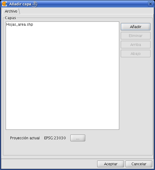
Figure 12: Add layer
Then the dialog CRS and transformation will open where you can select the CRS for the layer, and, if needed, a transformation to load the layer into the view (see figure 13).

Figure 13: Selection of the CRS for a layer
Compared to the New CRS dialog that was described before, what is new here is that the table of used CRS includes a Transformation column. This column facilitates the simultaneous selection of the CRS and the transformation for a layer, but only if these have been used before.
The selection of a transformation will be described hereafter.
The CRS for the View must be defined through the dialog View properties which can be accessed by clicking on the Properties button in the Project manager of gvSIG (see figure 9).
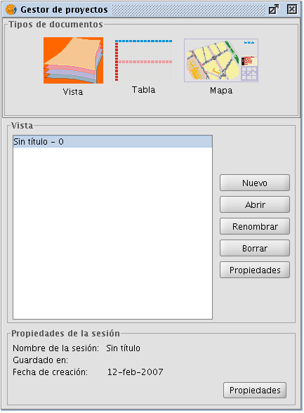
Figure 9: Project manager of gvSIG
After clicking on the Current projection button of the View properties dialog (see figure 10), the New CRS dialog will open (see figure 11) which has been described in the previous section.
IMPORTANT: Currently it is not possible to re-project an open view, so if you change the CRS while the view is open, the results may be erroneous.
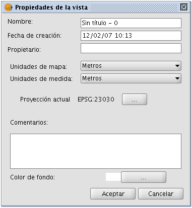
Figure 10: View properties dialog

Figure 11: Selection of the CRS
This section describes how to set the default CRS for every new View that is created in gvSIG.
The default CRS is defined in the Preferences window of gvSIG which can be accessed through the menu (Window->Preferences) or with the corresponding button in the toolbar  , see figure 1.
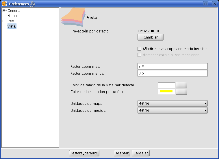
Figure 1: View Preferences
When clicking on the Change button, the New CRS dialog is displayed which lets you select the default CRS, see figure 2.
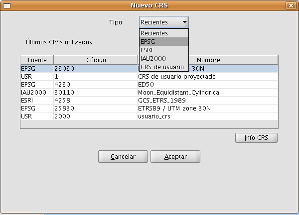
Figure 2: Select CRS. Recent CRS
In this dialog you can select CRS from five different repositories:
- Recent: This includes the CRS that have been used previously (Figure 2). The list of recent CRS will be available in the current and future executions of gvSIG and is not linked to a specific project.
- EPSG: This lets you browse and select CRS from the EPSG (European Petroleum Survey Group) database.
- ESRI: This lets you browse and select CRS from the ESRI database
- IAU2000: This lets you browse and select CRS from the IAU2000 database.
- User CRS: With this option you can create or select a user-defined CRS. When creating a new user-defined CRS, you can base this CRS on existing CRS from the EPSG database or create it from scratch.
Below, a brief description of each option is presented.
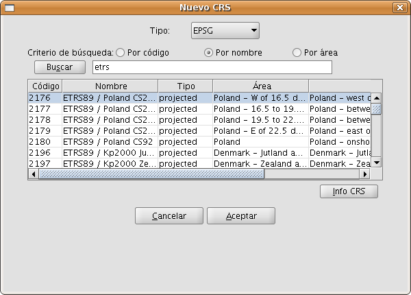
Figure 3: EPSG repository
The selection of CRS from the EPSG database can be done through three search criteria: through the EPSG code (for example 4230), through the name of the CRS (for example ETRS89), or by the area where the CRS is used (for example Spain). The two last cases are character string searches, resulting in those CRS where the name or area description includes the introduced string.
By clicking on the Info CRS button, you can access detailed information about the CRS that is selected in the table at the moment when you click the button, see figure 4 and 5:
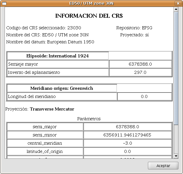
Figure 4: Information of the selected CRS
In the information that is shown for the selected CRS, it is important to note the Proj4 string (at the bottom). The jCRS library includes CRS operations through the Proj4 library (link), where the results will be correct if this string has been correctly constructed. This information could be useful for advanced users.
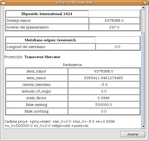
Figure 5: Information of the selected CRS, including the proj4 string
This information sheet for selected CRS is available for all repositories included in the extension.
The selection of CRS from the IAU2000 and ESRI databases, (see figure 6 and 7, respectively) can be done by searching on the CRS code or name of the CRS.
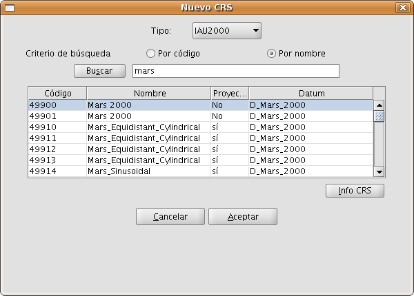
Figure 6: IAU2000 repository
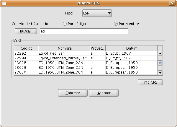
Figure 7: ESRI repository
The User CRS dialog allows for the management of the user database including select, edit or delete existing CRS, or create new CRS.
The selection of existing user-defined CRS (see figure 8) can be done by searching on the CRS code or the name of the CRS. Since there are normally only a few user-defined CRS, all user-defined CRS will appear in the table by default when the New CRS dialog is opened or when a search is performed without any code or search string.
The process of creating, editing and deleting of user-defined CRS will be explained in a later section of this manual.

Figure 8: Repository of user-defined CRS
In accordance with ISO 19111, there are two types of operations to relate two different CRS: conversion operations and transformation operations:
- Conversion of coordinates is used when the datum of the CRS of the layer coincides with the datum of the CRS in the view, in other words, both CRS correspond to the same geodetic reference system but are in different coordinate systems. If you choose the CRS of the layer in this case you need to select the option No transformation.
- Transformation is used when the datum of the CRS of the layer does not coincide with the datum of the CRS of the view. In this case there are two types of coordinate operations:
- The operation involves only a transformation when the coordinate system of the CRS of the layer coincides with the coordinate system of the view; in both CRS the positions are expressed in the same coordinate system but in a different datum.
- The operation involves a transformation and a coordinate conversion when both the datum and the coordinate system of the CRS of the layer and the CRS of the view are different.
If a transformation is needed, you must choose the type of transformation for the layer in the CRS selection dialog (see Figure 20) and click the Next button to continue to the corresponding transformation dialog.
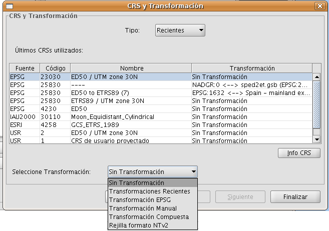
Figure 20: Select the type of transformation
The transformation dialog depends on the type of transformation to be performed:
- EPSG transformation. These are the official 7-parameter transformations as defined in the EPSG repository. The dialog for this type of transformation shows a table where all the applicable EPSG transformations are listed, with the CRS that was chosen for the layer as source CRS, and the CRS of the View as destination CRS (see Figure 21).
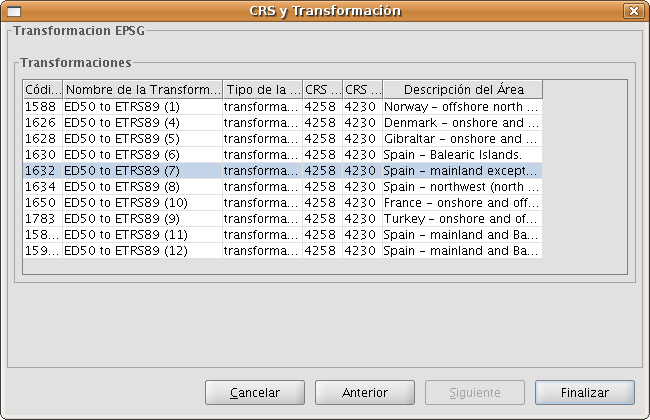
Figure 21: Transformación EPSG
Keep in mind that the transformation operations of this type are always between the base CRS (i.e. non-projected CRS), and therefore if the CRS of the view or the CRS of the layer is projected, the corresponding base CRS will appear in the fields Source CRS and Destination CRS. Keep also in mind that for this type of transformation, the CRS for the View and the CRS for the layer must come from the same EPSG repository. If they come from different repositories, the table will appear empty.
- Manual transformation. With this option you can define a Helmert transformation through the introduction of the 7 parameters (see Figure 22).
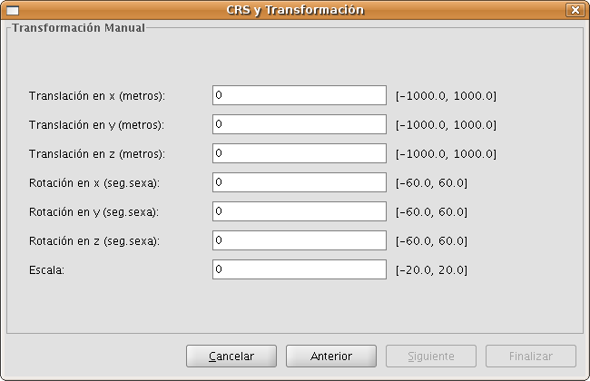
Figure 22: Manual transformation
- Grid based transformation (see Figure 23). With this option a transformation based on an NTv2 grid file is applied. For this, you must choose the NTv2 file from a list of available files or import it from a location to be specified. Since in the NTv2 file the translations have been calculated in a given base CRS, you must indicate here whether the NTv2 was calculated in the base CRS of the View, or the base CRS of the layer.
IMPORTANT: The grid file has a specific scope, which can be deduced from the file information that is displayed in the processing panel. Transformation is not applied beyond this scope, so the re-projection accuracy will be considerably lower, since only the corresponding coordinate system conversion would be applied.
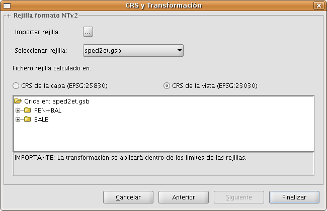
Figure 23: Grid based transformation
Recent transformations (see Figure 24). With this option, you can select a transformation that has been used before. The list of recent transformations will be available in the current and future executions of gvSIG and is not linked to any specific project.
There are two ways to select a recent transformation. The first way is through the CRS selection panel for the layer. There is now an additional field in the table to indicate if the selected CRS has been used together with a transformation in any recent execution of the program. If you select the CRS and recent transformation, you can do two things:
- Accept the CRS and transformation.
- Continue the process of selecting the transformation. This will be helpful to review the selected transformation, because in the next panels the information of the selected transformation will be loaded, so that you can still change it or select another transformation, in which case in the next CRS selection for the layer, a new recent transformation will be added with the chosen settings. To access the information of the CRS and the transformation, just click on the Info CRS button (see Figure 25).
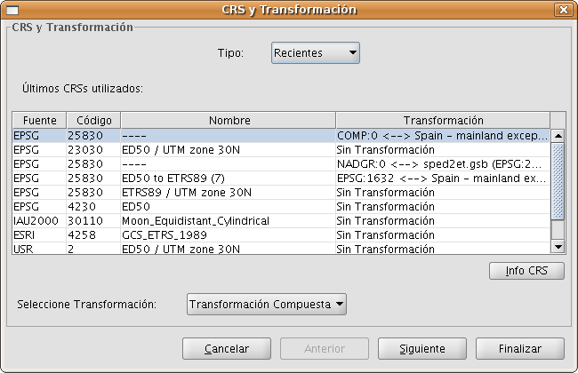
Figure 24: Selection of the CRS for the layer and recent transformation
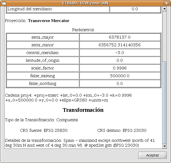
Figure 25: Information of the CRS for the layer and the selected transformation
The second way to select a recent transformation is through the selection of CRS without transformation and then select Recent transformations as the type of transformation, after which a panel is displayed where you can choose from transformations that were previously defined (see Figure 26).
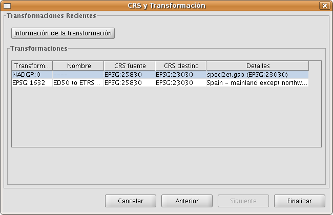
Figure 26: Recent transformations
Composite transformation. This type of transformation is new for this version. The objective of composite transformations is to provide gvSIG users with the possibility to represent two CRS with different datums without the transformation between those two CRS, but with a transformation of those two CRS into a third CRS.
The composite transformation can play an important role when you need to define two transformations, one that refers to the CRS of the layer and the other to the CRS that has been defined for the view.
With this mechanism, you can set the CRS for the layer and the CRS of the View through an intermediate CRS that connects the two CRS.
To do this, after selecting the CRS of the layer and setting the type of transformation to Compound transformation, you need to:
- Define the transformation to be applied to the CRS of the layer (Figure 27)
- Define the transformation to be applied to the CRS of the view (Figure 28).
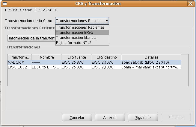
Figure 27: Select the transformation for the CRS of the layer

Figure 28: Select the transformation for the CRS of the view
Raster
Adding a layer from a disk file
Click on the "Add" button
The "Add” dialogue window allows you to move around the file system to select the layer to be loaded. Remember that only the files of the type selected will be shown. To indicate the type of file to be loaded, select a file from the “Files of type” pull down menu.
If several layers are loaded at the same time, the order in which the themes will be added to the view can be specified with the "Up" and "Down" buttons in the “Add layer" dialogue.
Adding a layer using the WMS protocol
Go to the "Add layer" window and then select the WMS tab.
- The pull-down menu shows a list of WMS servers (you can add a different server if you don’t find the one you want).
- Click on “Connect”.
- and 4. When the connection is made, a welcome message from the server appears, if this has been configured. If no welcome message appears, you can check whether you have successfully connected to the server if the “Next” button is enabled.
- The WMS version number that the connection has been made to is shown at the bottom of the box.
Click on “Next” to start configuring the new WMS layer.
When you have accessed the service, a new group of tabs appears.
The first tab in the adding a WMS layer wizard is the information tab. It summarises the current configuration of the WMS request (service information, formats, spatial systems, layers which make up the request, etc.). This tab is updated as the properties of its request are changed, added or deleted.
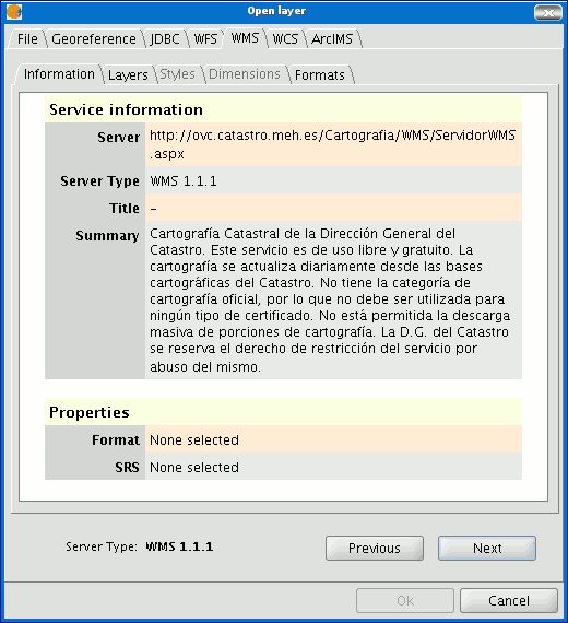
The wizard’s “Layers” tab shows the WMS server’s table of contents.
Select the layers you wish to add to your gvSIG view and click on “Add”. If you wish, you can choose a name for the layer in the “Layer name” field.
N.B. Several layers can be selected at the same time by holding down the “Control” key and left clicking on the mouse.
N.B. To obtain a layer description move the cursor over a layer and wait a few seconds. The information the server has about these layers is shown.
The “Styles” tab allows you to choose a display view for the selected layers. However, this is an optional property and the tab may be disabled because the server does not define styles for the selected layers.
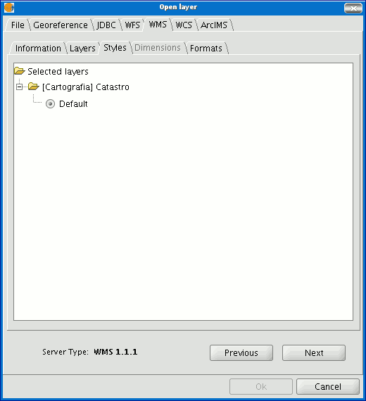
The “Dimensions” tab helps to configure the value for the WMS layer dimensions. However, the dimensions property (like the styles property) is optional and may be disabled if the server does not specify dimensions for the selected layers.
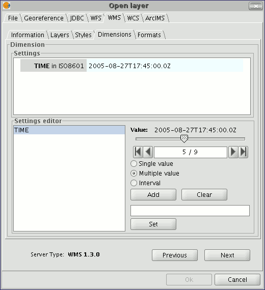
No dimension is configured by default. To add a dimension, select one from the “Settings editor” area in the list of dimensions. The controls in the bottom right-hand corner of the tab are enabled. Use the slider control to move through the list of values the server has defined for the selected dimension (for example “TIME” refers to the dates the different images were taken). You can move back to the beginning, one step back, one step forward or move to the end of the list using the navigation buttons which are located below the slider control. If you know the position of the value you require, you can simply write it in the text field and it will move automatically to this value.
Click on “Add” so that you can write the selected value in the text field and request it from the server.
gvSIG allows you to choose between:
Single value: Only one value is selected
Multiple value: The values will be added to the list in the order they are selected in
Interval: An initial value and then an end value are selected
When the expression for your dimension is complete, click on “Set” and the expression will appear in the information panel.
N.B. Although each layer can define its own dimensions, only one choice of value is permitted (single, multiple or interval) for each variable (e.g. for the TIME variable a different image date value cannot be chosen in each layer).
N.B. The server may come into conflict with the layer combination and the variable value you have chosen. Some of the layers you have chosen may not support your selected value. If this occurs, a server error message will appear.
N.B. You can personalise the expression in the text field. The dialogue box controls are only designed to make it easier to edit dimension expressions. If you wish you can edit the text field at any time.
The “Formats” tab allows you to choose the image format the request will be made with, specify if you wish the server to hand in the image with a transparency (to superimpose the layer onto other layers the gvSIG view already contains) and also the spatial reference system (SRS) you require.
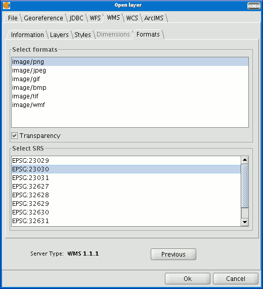
As soon as the configuration is sufficient to place the request, the “Ok” button is enabled. If you click on this button, the new WMS layer will be added to the gvSIG view.
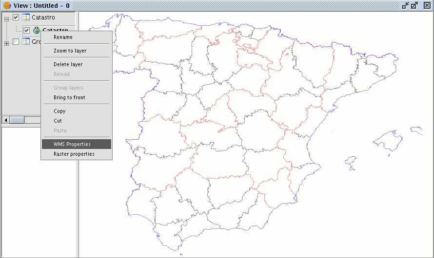
Once the layer has been added its properties can be modified. To do so, go to the Table of contents in your gvSIG view and right click on the WMS layer you wish to modify. The contextual menu of layer operations appears. Select “WMS Properties”. The “Config WMS layer” dialogue window appears. This is similar to the wizard for creating the WMS layer and can be used to modify its configurations.
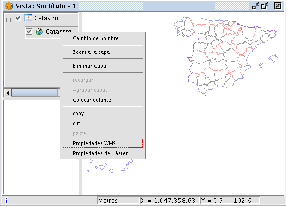
Adding a layer using the WCS protocol
Click on “Next” to start configuring the new WCS layer.
When you have accessed the service, a new group of tabs appears.
The first tab in the adding a WCS layer wizard is the information tab. It summarises the current configuration of the WCS request (service information, formats, spatial systems, layers which make up the request, etc.). This tab is updated as the properties of its request are changed, added or deleted.
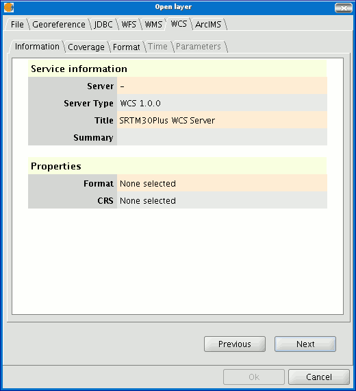
Select the coverage you wish to add to your gvSIG view. If you wish, you can choose a name for your layer in the “Coverage name” field.
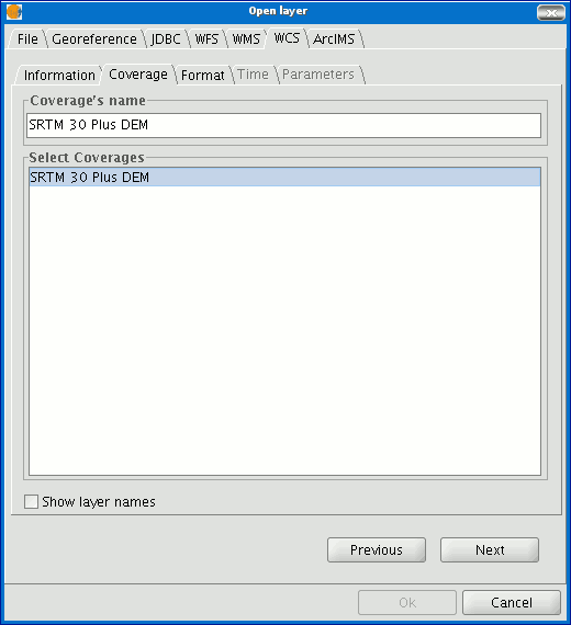
You can choose the image format you wish to use to make the request and reference system (SRS) in the “Format” tab.
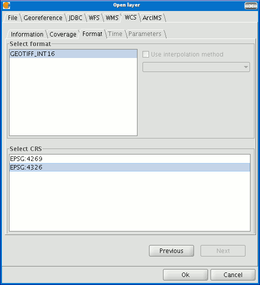
N.B. Tabs such as “Time” and “Parameters” are disabled in this case. Configuring these variables depends on the server chosen and the type of data it has access to.
As soon as the configuration is sufficient to place the request, the “Ok” button is enabled. If you click on this button, the new WCS layer will be added to the gvSIG view.
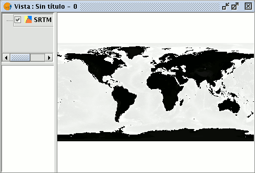
Once the layer has been added its properties can be modified. To do so, go to the Table of contents in your gvSIG view and right click on the WCS layer you wish to modify. The contextual menu of layer operations appears. Select “WCS Properties”.
The “Config WCS layer” dialogue window appears. This is similar to the wizard for creating the WMS layer and can be used to modify your configurations.
Adding orthophotos using the ECWP protocol
If you wish to add an orthophoto to gvSIG using the ECWP protocol, first open a view and click on the “Add layer” button.

Click on the “Add” button in the dialogue box. A file browser window appears.
Choose the “gvSIG Image Driver” option from the “Files of type” pull-down menu.
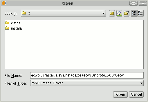
Write the URL of the file you wish to load as follows in “File name”:
ecwp://server address/path of the file you wish to add.
For example:
ecwp://raster.alava.net/datos/ecw/Ortofoto_5000.ecw
ecwp://earthetc.com/images/geodetic/world/MOD09A1.interpol.cyl.retouched.topo.bathymetry.ecw
When you have input the data, click on “Open”.
The orthophoto will be added to the layer list.
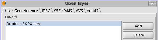
Select the new added layer and click on “Ok”.
The image will be added to the view.
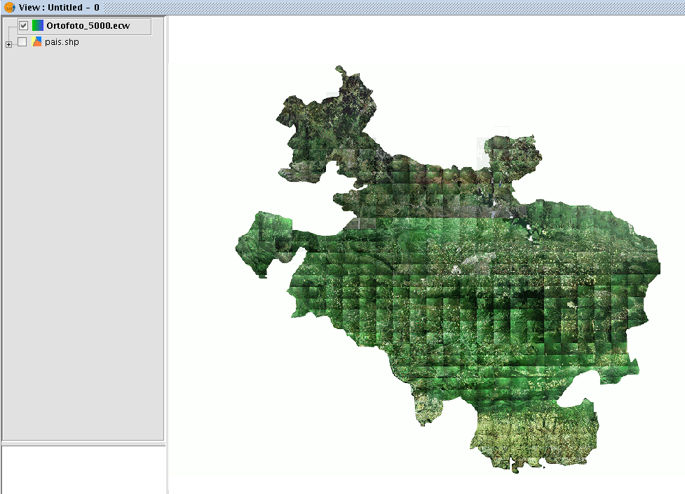
Adding a layer using the ArcIMS raster
In the proprietary software environment, ArcIMS (developed by Environmental Sciences Research Systems, ESRI) is probably the most widespread/popular widely used (Internet) cartographic server on the Internet thanks to the number of clients it supports (HTML, Java, ActiveX controls, ColdFusion...) and to its integration with other ESRI products. ArcIMS is currently one of the most important remote cartographic information providers. Although the protocol it uses does not comply with the Open Geospatial Consortium (because it was created long beforehand), the gvSIG team believes that offering support for ArcIMS is important.
The extension can access image services offered by an ArcIMS server. This means that, just like a WMS server, gvSIG can request a series of layers from a remote server and receive a view rendered by the server containing the requested layers in a specific coordinate system (reprojecting if necessary) and in specific dimensions. In addition to displaying geographic information, the extension allows you to request information about the layers for a particular point via the gvSIG standard information button.
ArcIMS is slightly different in its philosophy from WMS. In WMS, the request is normally made by independent layers whilst in ArcIMS the request is global.
The steps required to request a layer from an ArcIMS server and to request information for a particular point are listed below.
Our example uses the ESRI ArcIMS server. Its URL is http://www.geographynetwork.com. This is the address a web browser requires to access the HTML visual display unit.
Before loading a layer from this server, the datum WGS84 in geodesic coordinates (code 4326) has to be set up previously as the view’s spatial system.
If the extension is loaded correctly, a new ArcIMS data source will appear in the “Add layer” dialogue box.
Adding a new layer to the view
If the server has a standard configuration, simply indicate its address. gvSIG will try to find the servlet’s full address.1 If the servlet has a different path, you will have to write it into the dialogue box.
When the connection has successfully been made, the server version, its compilation number and a list of image and geometry services available are shown.
The service can be selected from the list or can be written in directly.
Finally, if the “Override service list” check box is enabled, gvSIG will delete any catalogue that has already been downloaded and will request them again from the server.
List of services available
The next step is to select the ImageServer type service required by double clicking or selecting it and clicking on "Next". The dialogue box changes and an interface with two tabs appears (fig. 3). The first tab shows the metainformation given by the server about the service’s geographic limits, the acronym of the language it has been written in, units of measurement, etc. It is a good idea to find out if a coordinate system has been defined in the service (using EPSG codes) as this can directly influence the requests made to the server, as Figure 3 shows.
N.B. If no coordinate system has been defined in the service, the extension will assume that it is the same coordinate system as the one we have defined for the view.
Figure 3: Metadata from the ArcIMS server
We can continue by clicking on "Next" or return to the previous dialogue by clicking on "Change service”.
The last dialogue box is the layer selection. We can define a name for the gvSIG layer or leave the default value (the service name) in this window. A box appears below with a list of the service layers in tree form. When the mouse is moved over the layers, information about these layers appears: extension, scale ranges, type of layer (raster or vector image) and if it is visible by default in the service (fig. 4).
Figure 4: Metadata from a service layer
We can view each layer’s ID via the “Show layer ID” check box. This check box is useful when there are layers whose descriptor is repeated. Therefore, the only way to distinguish between them is via an ID, which will always be unique. A combo box is also available to select the image format we wish to use to download the images. We can choose JPG format if our service works with raster images or one of the other remaining formats if we want the service to have a transparent background.
N.B. The transparency in 24-bit PNG images is not correctly displayed in gvSIG 0.6. This type of files will be supported in gvSIG 1.0.
The box with the layers selected for the service appears below. If you wish, you can add just some of the service layers and also reorganise them. This makes the service view totally personalised.
N.B. The configuration cannot be accepted until a layer has been added.
N.B. Multiple selections of service layers can be made by using the Control and CAPS keys.
When the “Ok” button in the dialogue box is pressed, a new layer appears in the view (fig. 5). If no layer has been added previously, the extension of the ArcIMS layer is shown, as per the standard gvSIG procedure.
Figure 5: ArcIMS layer added to the gvSIG view.
It must be remembered that when the layer extension is shown, the layers that make up the chosen configuration may not appear and a blank or transparent image appears instead. If this occurs, use the scale control dialogue box (V. Information about scale limits section).
An ArcIMS server does not define the spatial reference systems it supports as opposed to the WMS specification. This means that a priori we do not have a list of EPSG codes that the map server can reproject. In short, ArcIMS can reproject to any coordinate system and leaves the responsibility of how the projections are used to the client.
Therefore, if our gvSIG view is defined in ED50 UTM zone 30 (EPSG:23030) and we request a global coverage service (stored for example in the geographic coordinates WGS84, which correspond to code 4326) the server will not be able to reproject the data correctly because we are using global coverage for a projection of a specific area of the Earth.
However, the procedure can be carried out in reverse. If we have a view in geographic coordinates (and thus global coverage), services defined in any coordinate system can be requested because the server will be able to transform the coordinates correctly.
In short, requests to the ArcIMS server must be made in the view's coordinate system and they cannot be requested in another coordinated system.
Moreover, as we mentioned above, if an ArcIMS server does not offer information about the coordinate system its data is in, the user will be responsible for setting up the correct coordinate system in the gvSIG view. Thus, if a user with a view in UTM adds a layer which is in geographic coordinates (even though the server does not show it), the service will be added correctly but will take the view to the geographic coordinates domain (in sexagesimal degrees).
An additional effect is that if the view uses different units of measurement from the server, the scale will not be shown correctly.
The layers requested from the server can be modified via a dialogue box, which can be accessed from the layer’s contextual menu (fig. 6) just like the WMS layers. This dialogue box is similar to the box used to load the layer, apart from the fact that the service cannot be changed.
Figure 6: Properties of the ArcIMS layer
The extension allows us to consult the layers' scale limits which make up the requested service via a dialogue box which can be maintained in the view during the session (fig. 7). This window shows the layers on the vertical axis and the different scale denominators on the horizontal axis via a logarithmic scale. This box is small on screen but can be enlarged to improve the difference between the scales.
The vector layers, raster layers and the layers that can be seen on the current scale (marked with a vertical line) in a darker colour and the layers we cannot see above or below the current scale are differentiated by different coloured bars (described in the window legend).
Figure 7: Scale limits status
Attribute information requests about the elements for a particular point is one of gvSIG’s standard tools. Its functionality is also supported by the extension.
The WMS specification allows information about several layers to be requested from the server in one single query. This is different in ArcIMS. We need to make one server request per layer required.
This means that no requests for unloaded layers or unseen layers that are not visible on the current scale or layers whose extension is outside the view will be made. Even if all these layers are filtered, the information request usually takes longer than is desirable because of this intrinsic feature of ArcIMS.
When all the request responses have been recovered, the standard gvSIG attribute information dialogue appears with each of the layers (LAYER) which return information as a tree. If we click on a layer, its name and ID appear on the right (fig. 8).
Under this node, if we are talking about a vector layer, all the records or geometric elements the server has responded to appear, and give each one their corresponding attributes (FIELDS).
If it is a raster layer, such as an orthoimage or a digital terrain model, it returns the values for each of the bands (BAND) in the requested pixel colour, instead of records.
Figure 8: Displaying attribute information
The extension allows access to both ArcIMS image services and geometry services (Feature Services). This means that a server can be connected to and geometric entities (points, lines and polygons) and their attributes obtained. This is not dissimilar to WFS service access.
However, the variety of existing geometry services is much lower than the variety in the image server. There are two main reasons for this. On one hand, providing the public with vector cartography implies security problems because many bodies only want to offer the general public views and images. The vector data becomes either an internal product or must be paid for. On the other hand, this type of services generate much more traffic on the network and in the case of basic information servers could become a problem.
Loading a geometry layer is practically the same procedure as loading the image server as mentioned above (Accessing the service section and the following sections). In this case, the number of layers to be selected must be taken into account. If we wish to download all the layers offered by the service the response time will be very high.
The only difference between loading an image layer is that in this case we can choose whether we wish the layers to be downloaded as a group via a check box. This is useful for processing the vector layers as one layer when it needs to be moved and activated in the table of contents.
Unlike the image service, in which all the service’s layers appear as one unique layer in the gvSIG view, in this case each layer is downloaded separately and appears in the view grouped under the name defined in the connection dialogue.
Cartography symbols are configured in the server in one AXL extension file for both geometry and image services. We can divide symbol definition into two parts. On one hand, we can talk about the definition of the symbols themselves, i.e. how a geometric element, such as a line or polygon, should be presented. On the other hand, we can talk about the distribution of these symbols according to the cartographic display scale or to a specific theme attribute.
In ArcIMS terminology symbols are different from legends (SYMBOLS and RENDERERS).
There are various types of symbols: raster fill symbols, gradient fill symbols, simple line symbol, etc. The extension adapts the majority of the symbols generated by ArcIMS. Table 1 shows the ArcIMS symbols and indicates whether they are supported by gvSIG.
| Label | Description | Supported |
|---|---|---|
| CALLOUTMARKERSYMBOL | Balloon-type label | NO |
| CHARTSYMBOL | Pie chart symbol | NO |
| GRADIENTFILLSYMBOL | Fill in with gradient | NO |
| RASTERFILLSYMBOL | Fill with raster pattern | YES |
| RASTERMARKERSYMBOL | Point symbol using pictogram | YES |
| RASTERSHIELDSYMBOL | Customised point symbol for US roads | NO |
| SIMPLELINESYMBOL | Simple line | YES |
| SIMPLEMARKERSYMBOL | Point | YES |
| SIMPLEPOLYGONSYMBOL | Polygon | YES |
| SHIELDSYMBOL | Point symbol for US roads | NO |
| TEXTMARKERSYMBOL | Static text symbol | NO |
| TEXTSYMBOL | Static text symbol | YES |
| TRUETYPEMARKERSYMBOL | Symbol using TrueType font character | NO |
Table 1: ArcXML symbol definition labels
In general, the most common symbols have been successfully “transferred”. Some of the symbols cannot be obtained directly from gvSIG (at least in the current version), such as the raster fill symbol or they need to be “adjusted” such as the different types of lines. This means that a raster fill symbol is not a symbol that can be defined by the gvSIG user interface, but it can be defined by programming.
gvSIG supports the most common types of legends: unique value and range and value themes as well as the scale-range control over the whole layer. ArcIMS goes much further in its configuration. It can generate much more complicated legends in which symbols can be grouped together, scale-range controls can be established for labels and symbols and different labelling based on an attribute can be shown (as though it were a value theme for labelling).
This group of legends can generate very complex symbols for a layer in the end. The current implementation status of the gvSIG symbols needs to be simplified to reach a compromise to recover the symbols that best represent the layer as a whole.
| Label | Description |
|---|---|
| GROUPRENDERER | Legend which groups others together |
| SCALEDEPENDENTRENDERER | Scale dependent legend |
| SIMPLELABELRENDERER | Labelling layer legend |
| SIMPLERENDERER | Unique value layer legend |
| VALUEMAPRENDERER | Value and range themes |
| VALUEMAPLABELRENDERER | Labelling themes |
Table 2: ArcXML legend definition labels
When a GROUPRENDERER is found, the symbol ArcIMS draws first is always chosen. Thus, in the case of the typical motorway symbol for which a thick red line is drawn and a thinner yellow line is drawn over it, gvSIG will only show the red line with its specific thickness.
If a scale dependent legend is discovered during a symbol analysis, this is always chosen. If more than one is discovered, the one with the greatest detail is chosen. For example, in ArcIMS we can have a layer with simple road symbols (only main roads are drawn) on a 1:250000 scale and based on this a different theme is shown with all types of roads (paths, tracks, roads, etc.). In this case, gvSIG will show this last theme as it is the most detailed.
If a labelling legend is discovered during a symbol analysis, it will be saved in a different place and will be assigned to the selected definitive legend. In the case of the VALUEMAPLABELRENDERER label, only the legend of the first processed value will be obtained as a label symbol. The rest will be rejected.
In short, it is obvious that the failure to adapt the legends for gvSIG is a simplification process in which different legend and symbol definitions must be rejected to obtain a legend which is similar to the original as far as possible. It is to be expected that the gvSIG symbol definition will improve considerably so that it can support a larger group of cases in the future.
Working with the layer is similar to any other vector layer, as long as we remember that access times may be relatively high. The layer attribute table can be consulted, in which case the records will be downloaded successively as we display them.
If we wish to change the table symbols to show a unique value or range theme we must wait as gvSIG requests the complete table for these operations. On the other hand, the downloading of attributes is only carried out once per layer and session and therefore, this wait only occurs in the first operation.
In general, if our ArcIMS server is in an Intranet, it will be relatively fast to handle, but if we wish to access remote services we may be faced with considerable response times.
The main feature to bear in mind when working with an ArcIMS vector layer is that the geometries available at any given time are only the ones displayed. This is because we can connect to huge layers but only the visible geometries are downloaded. As far as gvSIG is concerned, the geometries shown on the screen are the only ones available and thus, if we export the view to a shapefile for example, are only a part of the layer.
Finally, we need to remember that to speed up the geometry downloads they are simplified to the viewing scale in use at any given time. This drastically reduces the amount of information downloaded as only the geometries that can actually be "drawn" are displayed in the view.
Loading a geometry layer is practically the same procedure as loading the image server as mentioned above (Accessing the service section and the following sections). In this case, the number of layers to be selected must be taken into account. If we wish to download all the layers offered by the service the response time will be very high.
Unlike the image service, in which all the service’s layers appear as one unique layer in the gvSIG view, in this case each layer is downloaded separately and appear in the view grouped under the name defined in the connection dialogue.
After a few seconds the layers appear individually but are grouped under a layer with the name we have defined for it.
The layer symbols are established at random. A pending feature is to recover the service symbols and configure them by default so that gvSIG can display the cartography as similarly as possible to how it was established by the service administrator.
Web Map Context
Web Map Context (WMC) is another OGC standard (http://www.opengeospatial.org) which can be added to the list of standards of this type supported by gvSIG.
It can reproduce a view made up of Web Map Services (WMS) layers on any GIS platform which supports WMC. If your project has a view which contains WMS layers, you can export these layers. The result is an XML file with a specific format and .cml extension which can be imported by another platform on which the view it describes can be reproduced.
Web Map Context (WMC) is another OGC standard (http://www.opengeospatial.org) which can be added to the list of standards of this type supported by gvSIG.
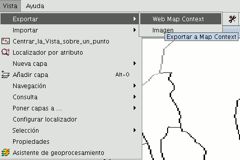
It can reproduce a view made up of Web Map Services (WMS) layers on any GIS platform which supports WMC.
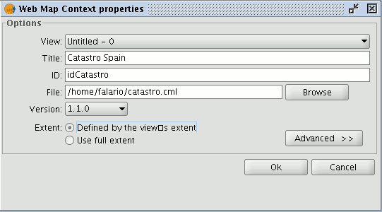
If your project has a view which contains WMS layers, you can export these layers. The result is an XML file with a specific format and .cml extension which can be imported by another platform on which the view it describes can be reproduced.
Exporting a view to WMC
Exports to WMC are currently limited to WMS type layers, although it is hoped that its functions will extend to all layers that comply with OGC standards in the future.
To obtain a WMC file, open a view in gvSIG and add the WMS layers you require.
Then go to the “View” menu and select “Export” and then “Web Map Context”.
The following dialogue will be shown.
N.B.: If you cannot find the "Web Map Context" option in the "Export" option, your project does not contain any WMS layers.
Basic mode only shows the compulsory properties which cannot be taken for granted by the application.
View: This defines which view is going to be exported to the WMC. The view which is currently active is selected by default.
Title: This is the title of the view which will be shown when your .cml file is loaded at a later date. The current title of the view is used by default but this can be changed.
ID: This field is also compulsory and represents a file ID which must be unique.
File: You can search for the place you wish to save the .cml file in from the "Browse" button.
Version: Use this tool to specify the WMC version you wish to use.
The version 1.1.0 is selected by default as it is the most highly developed and the most recommended. However, several applications and geoportals are often limited to a specific version.
gvSIG currently supports Web Map Context in its versions 0.1.4, 1.0.0 and 1.1.0.
Extent: This defines the extension of the map to be exported.
Defined by the view’s extent. This option only exports what we can currently see in the view.
Use full extent. This extension is better to use the full WMS layers depending on how their respective servers define them.
If you click on the “Advanced” button, the advanced configuration dialogue will drop down. This allows you to define more properties to obtain a complete WMC.
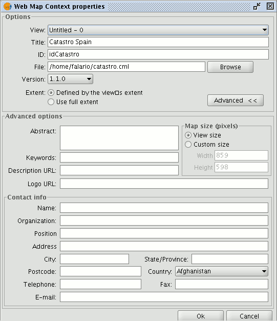
Abstract: This contains a summary of the view defined by WMC.
Keywords: This list of words allows you to classify and “metadata” the WMC.
URL description: If you have a web site which refers to this WMC, write its link here.
URL logo: If you have an image associated with this WMC, write its link here.
Map size (pixels): This defines the pixel size that the WMC-defined view will have. The current gvSIG view size is used by default but you can customise the size if you wish.
Contact info: Information that allows third parties to contact the WMC author.
Importing Web Map Context allows you to use gvSIG to open views with WMS layers which have been created with other platforms or with another gvSIG.
Use the "View” menu and select “Import” and then “Web Map Context”.
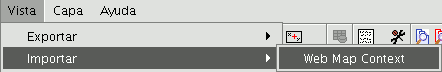
The WMC file selection dialogue opens.
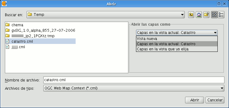
Choose the WMC file you wish to import. On the right, you can specify how you wish to view the layers.
New view: This adds a new view to the current project and loads the WMC as specified in the file.
Layers in the active (current) view: This option only appears if the active gvSIG window is a view. It allows you to quickly add the layers to the current view.
Layers in other view: This adds the layers defined by the WMC in the chosen view. In this option, a list of views appears to select the view that will contain the new layers.
Click on the “Open” button to import the file based on your preferences.
Alphanumeric data
File
Introduction
Tables are documents which contain alphanumeric information. Tables are made up of rows or records (which represent each of the elements in the data base) and columns or fields (which define the different attributes of each element).
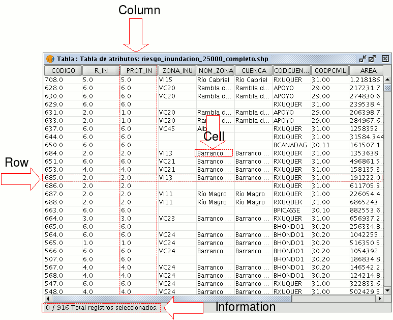
Row or record: Used to represent the different elements in the table.
Column or field: The types of attributes which define each element.
Cell: A cell is the intersection of a record and a field. A cell is the minimum working element and may contain information.
Record information: This provides information about the total number of elements (records) contained in the table.
All the vector information layers have their own “Table of attributes”. Each graphic element in a particular layer has its corresponding record in the “Table of attributes”.
To select elements in the table, left click on them. Use the “Control” and “Shift” (CAPS) keys to select more than one record.
Adding a Table
You can load a table in gvSIG in two ways:
- From the “Project manager”
- From the “View”
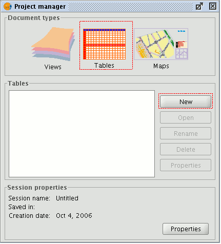
Select “Tables” as the document type from the “Project manager” and click on “New”. A dialogue box will open in which you can add the table.
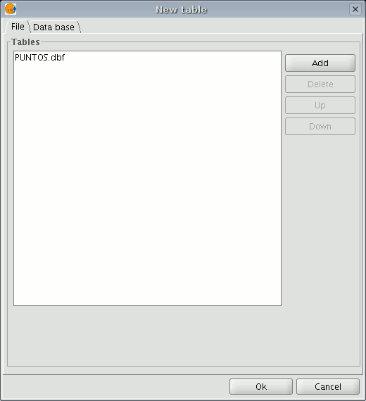
When you click on the “Add” button, a browser window will open.

Specify the type of file you wish to load in gvSIG in “Files of Type”. When you have located the file that contains the table, select it so that it is added to the “File name” text box and click on “Open”. You will automatically be returned to the "Add table" dialogue. If you wish to add more than one table, click on "Add" again and repeat the process. When you have finished, click on “Ok”. The table will then be displayed. It will also appear in the “Project manager” text box.
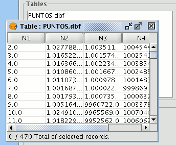
Click on the "See table of attributes" button from the display window of a view with at least one active layer, i.e. a layer that is selected in the ToC,

or go to the "Layer" menu and then select the "See table of attributes" option.
The table will automatically be added to the project.
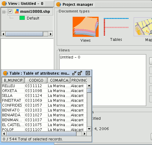
If you minimise the view, go back to the "Project manager" and select "Tables" as the document type, you will see that the table displayed in the view appears in the text box.
Table properties
You can access “Table properties” from the “Project manager” window.
You can use this window to:
- Rename the table.
- Edit the creation date.
- Add an owner to the table.
- Add comments.
When you have input the changes, click on “Ok” and they will be saved.
Table tools
When a table has been loaded, either from the “Project manager” or from the view, the tools associated with the table will appear in the tool bar.
A new menu, called “Table”, will also be activated in the tool bar. This can also be used to access the different tools.
You can access this option by clicking on the following button

or by going to the “Table” menu and then to “Statistics”.
The “Statistics” tool allows you to obtain the most common statistical values.
N.B.: Remember that the tool will not be activated until you select a numerical field.
If you wish to obtain field statistics, select the field (left click on the field heading), then click on the “Statistics” tool.
You can only obtain statistics from a series of records, firstly, select the field the values are located in, then select the desired records, and click on the “Statistics” tool.
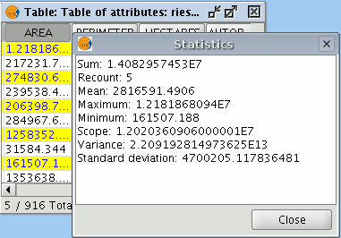
You can access this tool by clicking on the “Filter” button in the tool bar

or by going to the “Table” menu and then to “Filter”. The “Filter” tool works in much the same way as in the “Views” section.
gvSIG allows selections to be made using filters. Selection using filters allows you to define exactly what you want to select, including several attributes, operators and calculations.
Requests can be made using logical operators, such as “equals” “more than” “different from”, etc.
If you press the “Filter” button in the tool bar, a dialogue window will appear to define your request.

Fields: Double click on the field you wish to add to your request from the “Fields” list in the layer.
Logical operators: These allow you to insert a logical expression into your query by clicking on them.
Values: This shows a list with the different values the selected field has. If you wish to add a value to the request, double click on it.
Request: This is the window which represents the request to be made. You can write here directly.
Selection buttons: These buttons make the request using:
- “New set” (deletes any previous selections).
- “Add to set” (adds the elements selected by the query to the existing elements).
- “Select from set” (makes the request from the selected elements).
N.B.: In a gvSIG view, when you activate a layer by selecting it in the ToC, the filter tool will also be activated in the tool bar, even though no table has been loaded. This allows you to work with the table associated with the selected layer. The "Table" menu will also be added in the menu bar. This provides another way to access the filter tool when it drops down.
You can access this tool by clicking on the following tool bar button

or by going to the “Table” menu and then to “Ascending order”.
The “Ascending order” tool allows you to order the table records.
- It orders the values from the lowest to the highest in a numerical field.
- It orders the records in alphabetical order, starting from “A” in a text field.
You can access this tool by clicking on the following tool bar button

or by going to the “Table” menu and then to “Descending order”. The “Descending order” tool allows you to order the table records. It orders the values from the highest to the lowest in a numerical field. It orders the records in alphabetical order, starting from “Z” in a text field.
The “Join” tool allows two tables to be joined via a common field. You can also access this tool by clicking on the following button

or by going to the “Table” menu and then to “Join”. To join the two tables, carry out the following steps: Firstly, specify the source table the join is to be made from.
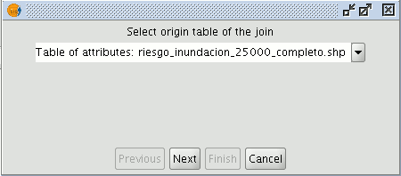
Then specify the field to be used for the join.
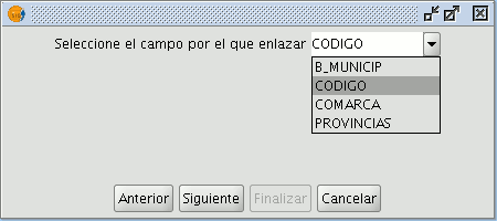
Then indicate the table you wish to join to the first one.
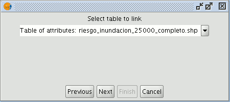
Finally, indicate the field in the second table which is common to the first one.
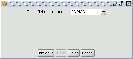
If you open the data source table, you will see that the fields of the destination table have been joined. The name of the field added to the table is identified by the word “Join_(Field name)”
This tool allows the records selected in the table to be moved to the top of the table. You can access this tool by clicking on the following button in the tool bar

or by going to the “Table” menu and then to “Move selection to top”. The following table shows an example in which two records have been selected to move to the top of the table.
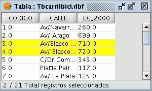
If you click on the button, the table will change the position of the selected records.
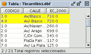
Although .dbf files should contain a byte to indicate character encoding, this information is usually not present. gvSIG provides the Shalom tool that sets the encoding and then reads the information in the table using that encoding. If the encoding is not set in this way then gvSIG will read the table data using the default encoding.
It is possible to set the character encoding of a table by selecting Table > Set encoding to .dbf files from the menu bar. Choose the table for which the encoding needs to be set and then select the encoding type (charset). This encoding setting is recorded permanently in the table.
Now the table can be added to the gvSIG project. When gvSIG opens the table the character encoding is read and the characters in the table are correctly displayed.
Note: The correct display of characters depends not only on the encoding setting, but also on the virtual machine that is installed (specifically Java 1.6, which supports more encodings than Java 1.5).
This option can be accessed by opening the Window > Preferences menu and then selecting DBF default encoding.
gvSIG will use the selected encoding as the default when adding a .dbf file to a project, and will also use it when exporting a table that uses a specific encoding.
The export of a table might not be correct if the character encoding is incorrectly configured in the gvSIG preferences.
Adding a table from a CSV file
From version 0.5 onwards, gvSIG can read information contained in a plain text file, whose fields are separated by a semi-colon.
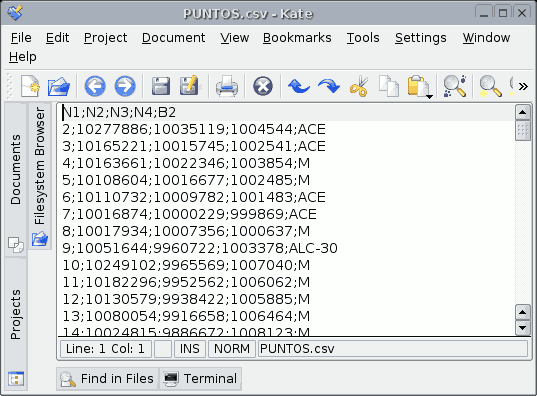
To carry out this operation, go firstly to the “Project manager”. Select “Tables” and then click on “New”. A search dialogue box will open. Click on “Add” and the file browser will appear in a new window (select “csv string” in “Type of file” to show the csv files).
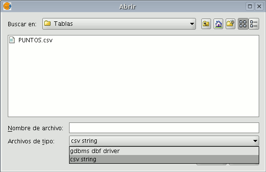
When the .csv file has been selected, click on “Open”.
If you click on “Ok”, the data of the table you have added will be shown.
Adding a table from a JDBC data origin
The contents of a data base table can be imported to gvSIG using data base managers (PostgreSQL, MySQL, GBMS-HSQLDB, ODBC). gvSIG processes the information obtained just like any other table.
Note: Oracle drivers installation is required for access to Oracle Spatial databases of the geoBD extension. Please follow the steps bellow: Go to Oracle Database 10g Release 2 (10.2.0.3) drivers.
Accept the license terms. In the next page, download the file ojdbc14.jar (1,545,954 bytes) - classes for use with JDK 1.4 and 1.5. (Registration required)
Move this file to the next folder:
- Windows:
Move the file to the:
bin\gvSIG\extensiones\com.iver.cit.gvsig\lib
folder, that is in the directory where gvSIG is installed.
- Linux:
Move the file to the:
bin/gvSIG/extensiones/com.iver.cit.gvsig/lib folder
, that is in the directory where gvSIG is installed.
To load a table with the information obtained from a JDBC data origin you must:
Firstly, go to the "Project manager" and select "Tables". Then click on "New". Select the “Data base” tab in the window that opens (“New table”) and configure the data base server connection parameters:
If the information entered is correct, a new table will be created in gvSIG with the information contained in the original JDBC table.
Symbology
Introduction
It is a tool which allows thematic cartography to be carried out with relative ease.
You can choose the colour, mesh etc. which most appropriately symbolises or represents the data or variables of the elements to a layer.
To access the edit option of properties related to the symbology you must go to the “Properties” menu (click on the smaller button on the layer).
Another window will open, place the cursor on the “'tables of symbols' tab".
Vectorial
Legends types
Introduction
In this tab you can define, in an advanced manner, the type of legend with which you want to represent the data of layer, from its fields [1].
[1]: It must be noted that you can not use the fields resulting from a join to make legend classifications, meaning that, to use these fields in a legend you will have to export the shp resulting from the join.
You can choose the following forms of representation:
Quantities
Four types of legends can be found:
Point density
Defines a legend of a point density based on the value of a certain field.
Labelling field A drop-down menu opens where you can choose fields from the table (Double or Integer types) from which you can make a legend which represents the quantity of each value in the table. The properties of the points which represent the density of the values in the table can be changed.
- Point size: Use the arrow to change size of the point.
Point value: This is the numeric value which will be given to each point that is drawn.
- Colour: Choose the colour of the point by clicking on the button located right of the colour.
- Background colour: Choose the background colour.
- Outline: Click on this button if you want to give an outline to the symbol.
Intervals
This type of legend represents the elements of a layer using a range of colours. The gaps or graduated colours are mainly used to represent numeric data which have progression or range of values, such as population, temperature, etc.
Classification field: A drop-down menu where you can chose the attributes of the layer for which you want to make the classification for. The field must be numerical as it is a gradual classification (by the rank of the value)
- Interval type: There are three types of intervals from which to choose. These are:
- Same intervals: Calculate same intervals from values which can be found in the chosen field to make the selection.
- Natural intervals: The number of intervals are specified and the sample of this number is divided into this number according to the Jenk method of optimisation of the natural localisation of intervals.
Cuantil intervals: The number of intervals are specified and the sample is divided into this number but gathering into groups values according to their order. Number of intervals: Should indicate the rank or interval number which defines their classification.
- Nº of intervals: Type in the nº of intervals to be represented.
- Initial and final Colour: Select the colours that will be used to graduate. The initial colour for lower values and the final colour for the higher ones.
- Calculating intervals: Once the above options have been defined, click on the “Calculate intervals” button to show the final result. The default symbols and labels that appear can be modified by clicking on them, just as in the previous cases.
- Add: New ranks to the calculations can be added.
- Remove all / Remove: Allows you to delete all (remove all) or some (remove) of the elements which make-up the legend.
Graduated symbols
Represents quantities through the size of a symbol showing relative values.
- Classification field: Choose the numeric field for which the classification is to be made.
- Interval types: The same that are in legend type Intervals
- Symbol: Modify the symbol size with a minimum value (From), to a maximum value (Until). You can also modify all the features of a specific symbol by clicking on the “Template” button, as well as its “background”.
- Calculating intervals: Once the above options have been defined, click on the “Calculate intervals” button to show the final result. The default symbols and labels that appear can be modified by clicking on them, just as in the previous cases.
- Add: New ranks to the calculations can be added.
- Remove all / Remove: Allows you to delete all (remove all) or some (remove) of the elements which make-up the legend.
Proportional symbols
Represents quantities through the size of the symbol which shows exact values.
- Classification field: Choose the numeric field for which the classification is to be made.
Normalisation fields: Possibility of choosing a numerical field which normalises the results, maintaining the proportion of quantities.
- Symbol: Modify the symbol size with a minimum value (From), to a maximum value (Until). You can also modify all the features of a specific symbol by clicking on the “Template” button, as well as its “background”.
Categories
Expressions
Shows layer elements according to a certain filtered expression.
- ''New filtered expression:'' A new window opens where you can configure expressions (filters) upon which a certain symbol will be applied. Each of these will be shown as a row in the main window of this type of legend. The syntax these filters use is SLD.
- ''Modification of filtered expression:''You are able to modify an expression by selecting it.
- ''Delete a filtered expression:''You are able to delete an expression by selecting it.
- ''Up/Down buttons:'' Allows you to move the created expressions up or down so that they later have that order in ToC.
Unique values
Each register can be represented with an exclusive symbol according to the value it adopts in a certain field in the attributes table. It is the most efficient method for spreading categorical data, such as municipalities, floor types, etc.

You will find the following symbology configuration options:
- ''Classification field:''A drop-down menu opens where you can select the layer which contains the data to carry out the classification, in the attributes table field.
- ''Add all/Add:'' Once the “classification field” is selected, all the different values are shown by assigning a symbol (colour) different to each by clicking on the “Add All” button. These symbols can be modified by clicking on them. By default the label (name that appears on the legend) is similar to the value that is adopted by this field. By clicking on “Add” you can add new values to the list.
- ''Delete all/Delete:'' Allows you to delete all (delete all) or some (delete) of the elements that make up the legend.
- ''Symbol properties:'' If you right click on any of the “cells” on the “Symbols” you can modify its properties specifically through the “Select symbol” and “Symbology level” buttons, as well as being able to change the label name in TOC.
Multiple attributes
Category quantities
Represents quantities for each category.
For this, it combines two fields (which must be of a numeric type), applying a combined legend made up of colour ramp (for field_1) and specific gradual symbols (for field_2).
Meaning that this type of legend combines a a representation of intervals based on the values of Field_1 with anothier representation of gradual symbols based on the values of field_2.
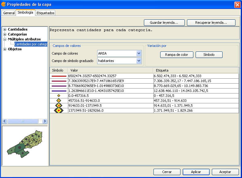
Objects
Unique symbol
This is the default gvSIG legend type.
Represents all the elements of a layer using the same symbols. It is useful for when you need to show the location of a layer more than its any other attribute. The representation of its symbology depends on the type of geometry, this is further explained in the symbols section.
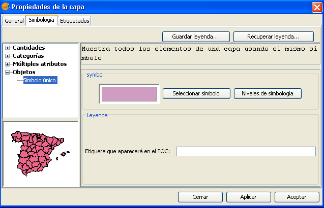
Saving and recovering legends
Save legend:
The legends that have been created can be saved so that you can use them on other occasions.
To save, click on the “Save legend” button.
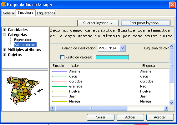
A window will open with the save options: save legend with gvSIV (.gvl) format or standard exchange .sld format (currently supports SDL 1.0.0).
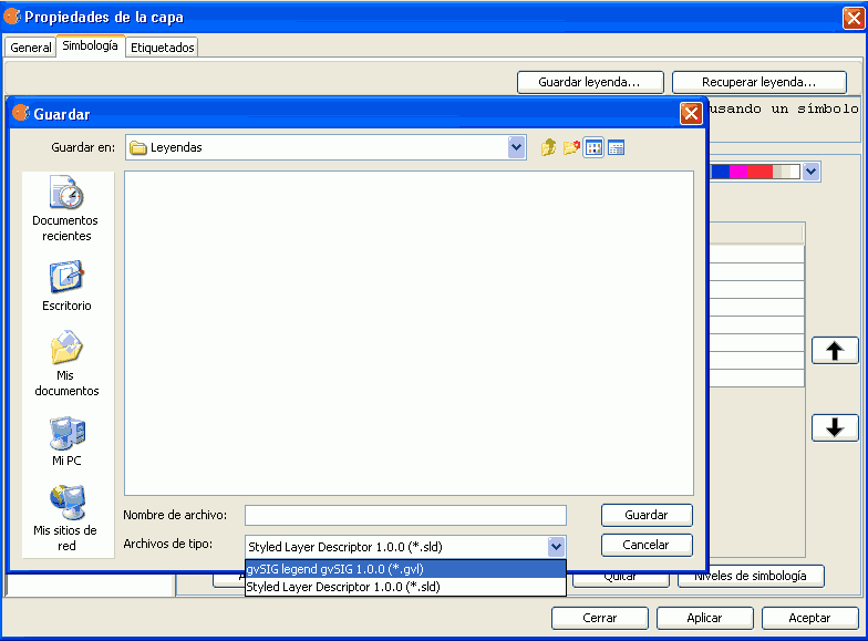
Legend recovery:
Legends that have been previously created can be recovered at any time. Click on the “Recover legend button” and select the legend you want to recover.
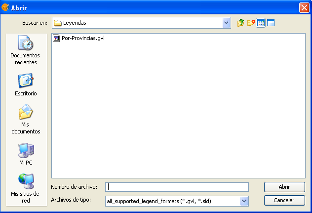
Modify symbols
Introduction
The Symbols tab is used to define advanced features of the legend being worked with.
When creating symbols for a legend it is important point to bear in mind the type of layer the symbols are being created for. This is important because there are two different types of vector layers to consider when making the symbols:
- Single geometry layers: (point, line or polygon shp layers). In this case the Symbols tab allows you to create or edit symbology relevant to the geometry (lines, points or polygons), as shown below:
Single geometry layer
- Multigeometry vector layers, such as dxf, dwg, gml ...
Multigeometry layer
In this case, there is a single Symbols tab where you can configure the symbol properties of the points, lines and polygons separately. Points are configured under the Marker tab, lines under the Line tab, and polygons under the Fill tab.
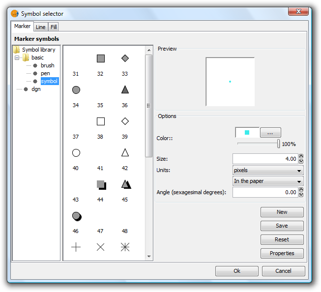
Tabs corresponding to the symbols for multigeometry layers
With this clarified, we can now look at symbol properties while taking the geometry type into account.
Symbol editor
From the layer menu, in properties, you can access the Symbology section. It is possible to change or configure a new symbol clicking on “Select symbol” where you will find different configuration options.
Click on the “Select symbol” button and then on the “Properties” button. The window which opens will allow you to edit the properties of the symbol. This is the same window that will open if you click on “New”.
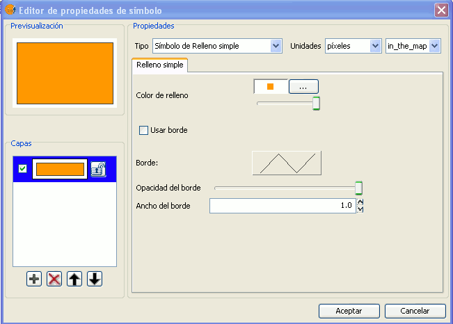
By default gvSIG symbolises the layers with 'unique symbols'.
As well as the basic options that can been seen at first glance, such as colour, breadth and the type of units in which the symbol is to be represented, you can also edit the properties of the element. Next a classification of the properties of an element is made according to its geometry type.
The dialogue boxes that open have common sections and others that are specific to the type of geometry, we see them as follows:
Common characteristics:
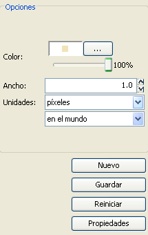
When a symbol, is configured from its Properties, be it a point, a line or a polygon, it can be defined:
- Its colour and transparency. Allows the fill-in colour to be chosen.
Under colour you find a scrolling bar, which allows you to play with the grade of the transparency of the elements. This way, you can superimpose polygon layers without interfering with its display.
- The breadth of the symbol. Allows you to define the breadth of the element.
- Units: In this drop-down menu you can chose the type of unit which you want the symbol to be represented in. By default the unit which the symbol will be represented in are pixels, although you can chose between: Kilometers, meters, centimeters, milimeters, miles, yards, feet, inches, grades and pixels.
We can also specify if they are units “on the map” (the size would depend on where the zoom is set) or “on paper” (it will have a set size, both on screen and when it is printed).
- New: Access the properties of the symbols in order to make a new symbol.
- Save: Allows you to save the symbols you have created in gvSIG's library of symbols, with a .sym extension, in order to be able to use them as often as you need and also to configure different types of legends.
- Restart: Click on this button if you wan to restart the editing of a symbol.
Specific characteristics of each type of geometry:
Symbol type:
| Mercator | Lines | Fill-in |
|---|---|---|
| Of character | Simple line | Simple fill-in |
| Simple mercator | Mercator lines | Image fill-in |
| Mercator image | Line image | Mercators fill-in |
| Of character | Simple line | Line fill-ins |
| Of character | Simple line | Gradient fill-ins |
The mercators represent the layers of the points.
The lines represent the linear layers.
The fill-ins represent the polygon layers.
All three together represent the multi-geometric layers.
You can chose between different Markers that are shown in “Type of Marker”.
Simple Marker:
In “Marker style”, select the marker (circle, square, cross...). You can modify its size, angle and colour as well as being able to move it around the ordinate and abscissa axis.
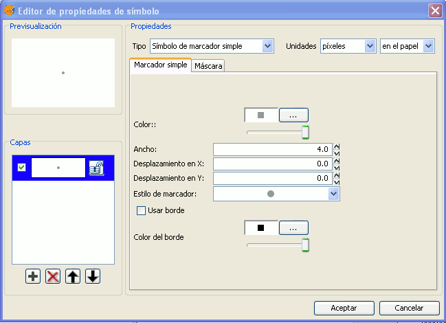
Marker made up of simple markers: you can make up a marker from various other simple markers by “overlapping” one over the other, this is done by clicking on “add layer”, where each layer is a simple marker. You can delete or change the order of the layers by clicking on “Delete layer” or “Tidy layers”. In the following image there is an example of a symbol made up of various simple markers.
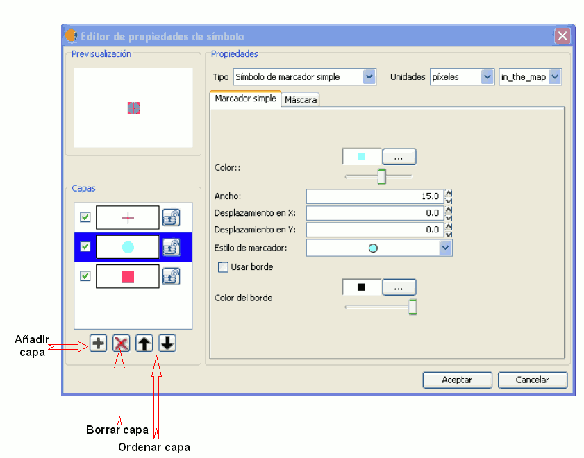
You can make the symbols stand out by choosing the colour of the outline and giving it the same transparency as the fill-in of the symbols. To give the symbol an outline you must check the “Use outline” box. You can move the symbol around the ordinate and abscissa axis or leave it in the centre.
Character marker:
You can use the different alphanumeric character types to create a symbol, you can modify its size, angle and colour as well as being able to move it around the ordinate and abscissa axis.
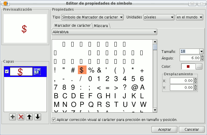
Picture marker:
You can chose whichever image you want to represent the symbol. This image can be in different formats (jpg, png,bmp, svg..., you can even download an image from the internet, as long as the format is supported by gvSIG). To add it just select the path where the image is saved by clicking on “Examine”, next to "Image file".
Also, you have the option of selecting a different image, which is to represent the geometries, when they have been selected and are in view. Do this by entering the path of the image in "Selected image".
You can move the symbol around the ordinate and abscissa axis or leave it in the centre.
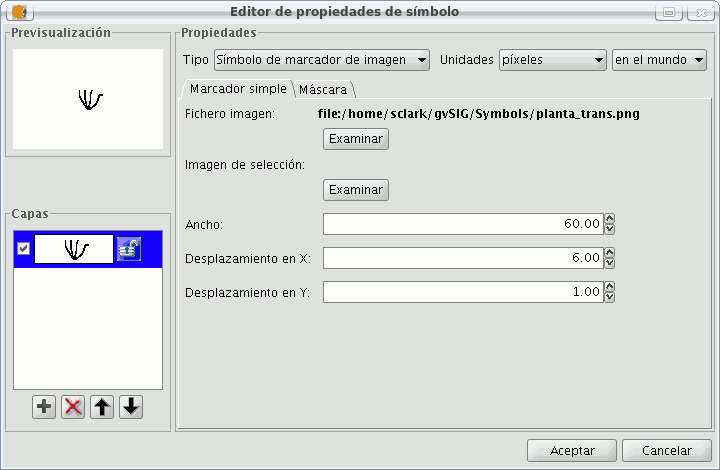
You can choose between different Mercator that are shown in the “Mercator type”.
Simple line symbol:
You can choose the colour of the line, its breadth and its movement (offset), as well as having the option to modify its opaqueness and, of course, its measurement units.
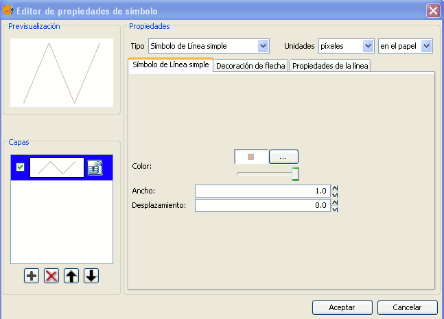
As well as that the layers of the points can make up one line with various lines “overlapping” using the same method than which in the layers of points.
In the “Line properties” tab you can generate different types of lines, continuous lines which gvSIG has as default, or discontinuous lines, establishing the fill-in pattern you choose. For this a rule is made available from which you can design your own patterns.
- Fill-in pattern:
Click on the grey section which is on the rule and drag right, next click on the rule, in the rule section you want, and a black section will appear which you can eliminate if you “click” on it again. This way you can successively add sections which can design your line.
If you want to delete the designed line click on “clean”.
- Boarder style: You can chose between round, rectangular or none for the boarder style.
- Style of the union: You can chose between square, angles and rounded for the union of the lines.
In the “Arrow decorations” tab you can turn a line into an arrow. To make this happen check the “Use decoration” box.
The options available to decorate the arrow are:
- The size of the arrow.
- The sharpness of the arrow.
- Nº of positions: Number of times you want the “point” of the arrow to be repeated along the line.
- Choose Symbol: This button will take you the simple Mercator of a layer of points menu, here you can select the shape of the arrow “point” and configure it as if it were any other symbol.
- Reverse: You have the option of reversing the first or all the arrows from the line.
- Rotation: You can chose between the “point” of the arrow rotates according to the slope of the line or that it has a permanent inclination according to the page.
Mercator line symbols:
You can use different font types, such as characters, to create a symbol, modifying its breadth and separation.
Image line symbol:
You can chose the image you want to make up the line, this image can be in different formats (jpg, png, bmp, svg...). To add the image you only have to select the path to where the image is saved by clicking on “Examine”. You can set the breadth and scale the image in “X” and “Y”.
The following fill-in Types for polygonal geometry layers are available.
Simple fill-in:
You can choose the polygon fill-in colour and its opaqueness.
Click on the button where you can see the outline and the simple symbol of a line properties menu will open. Here you can configure the outline of the polygon as if it were a line.
You can give the outline the breadth and opaqueness you want.
Fill-in made up of simple mercators: You can make up a fill-in from various simples by “overlapping” them, it is the same method as that which is explained in the layers of points and lines.
Mercator fill-ins:
You can give the polygon a fill-in made up of different types of mercators, such as punctual, linear, image... with their own characteristics.
The fill-in can be organised in an aleatory way or in a regular mesh way.
There is the option to make compositions with various layers.
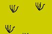
Line fill-in:
Instead of filling the polygon in with specific mercators you can do so with lines, you can give them the same properties that you gave a line layer, including the outlines.
As in all sections, here you can also create a composition through different layers.
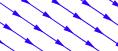
Image fill-in:
You can fill-in the polygon of images and set their inclinations by indicating the angle and you can also scale them.
The way to fill-in the polygon of images is by giving them the specific route to the image. These images can be framed, click on “Outline” and select the line you want.

Gradient fill-in:
The possibility of gradually filling-in is available, you can select different options to configure the gradual scale of the colour, these options are:
- Intervals: Nº of intervals you want the gradual changing of the colour to be structured by.
- Percentage: You can chose to set the percentage of gradual change between 0 and 100%.
- Style: Select the style that you want for the fill-in from the drop-down menu.
- Angle: Angle of the fill-in colour.
- Colour gradient: Select the colour scale you want.
- Outline: Give the ploygon an outline, the process of this is the same as if it were a line.
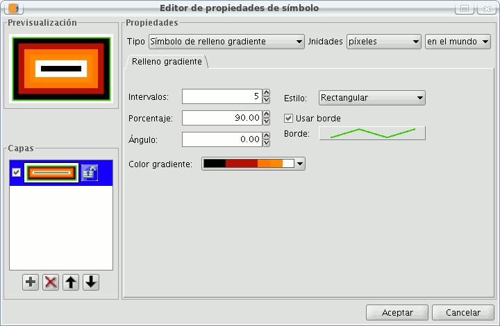
Symbol levels
As you can see in the following image, a symbol has two buttons that configure it, “Select Symbol” where you can define its properties, and “Symbology Levels” which allows us to establish the exact order the different layers has created the symbol.
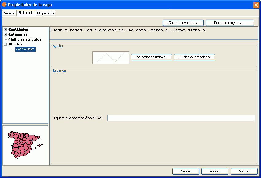
It is important to establish an order when different geometries of the same layer intersect, as can be the case in the unique Value of legends for line layers, for example, where the order established could be of interest so that some symbols are above others.
“0” value corresponds to the symbol drawn at that bottom, “1” is drawn above that and so forth successively.
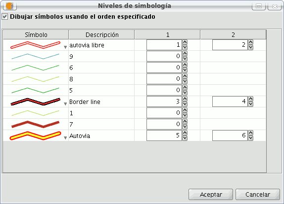
Labels that show in ToC
You can give whatever name you want to the different legend values, to see them in the Table of Contents.
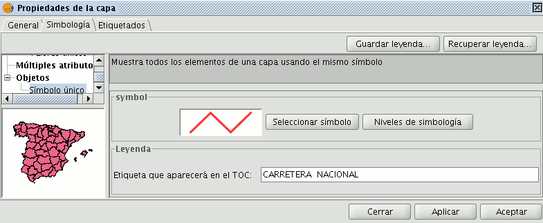
In the previous image we saw a legend by a unique Symbol, but it is also possible to give each of the legend values a label name by Interval, unique Value, etc. (or modify it, from each of the text boxes), as well as being able to modify the order with which theses values appear in ToC (throught the up/down arrows):
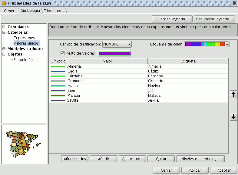
Library of Symbols
Upon installing gvSIC a folder called 'Symbols' is created in the user directory, here you can save different types of symbols (punctual, linear, polygonal...). In other words, it works as a library of symbols. Also, gvSIG includes, by default, a set of symbols from each type of geometry, saving them in the above mentioned folder.
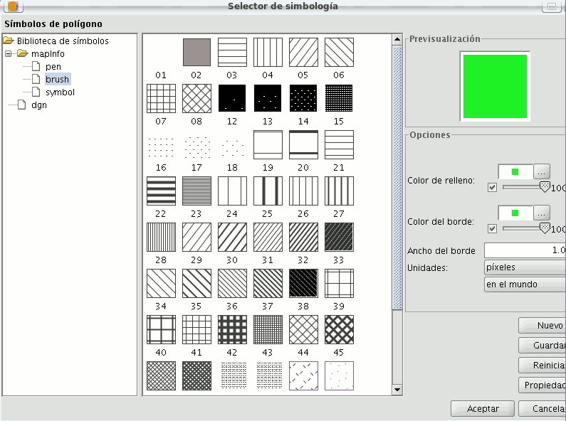
Once a symbol is created, from the “Symbology select” menu, click on “Save”.
A window will open, allowing you to save the symbols on a specific route, inside the “Symbols” folder.
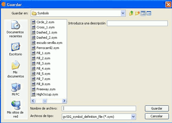
Name the symbol and click on save. Make sure you have saved the symbol as a .sym file and that when you open another layer of the same type of geometry, the library of symbols which has been saved appears.
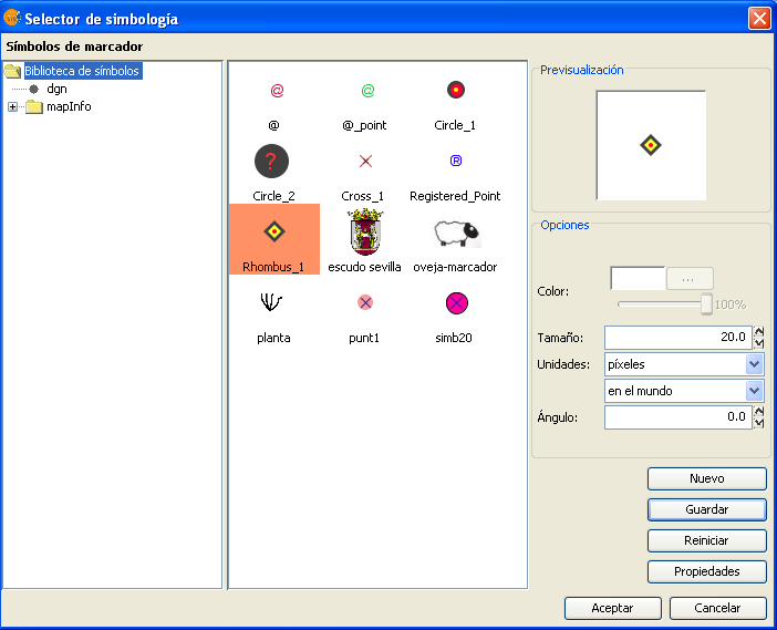
Raster
Color tables or gradients
The Colour table interface allows users to assign specific RGB values to a range of pixel values in a single band image. It is important to note that the input image can only have one band because if there are multiple bands, each of the bands will have colours associated with it. With the colour table functionality, users can build new tables or gradients, or modify existing ones.
The colour table dialog can be launched from the toolbar by selecting the option "Raster layer" on the left drop-down button and "Colour table" on the drop-down button on the right. Make sure that the name of the layer for which you want to build colour tables is set as the current layer in the text box. The "Colour table" option will only be available if a single band image is selected.

Colour table icon
To use this function, it is important to know the minimum and maximum values in the image. If these values are unknown, they will have to be calculated. Depending on the size of the image, this calculation process may take some time. When the Colour table dialog is launched for an image that does not have any colour tables associated with it, all components will be inactive. To get started, we need to tick the check box labelled "Activate color table".
Description of components
The colour table dialog is divided into several parts:
- The central part, which covers most of the dialog, displays the legend associated with the image in tabular or gradient form. (You can switch between table and gradient view by clicking on the tabs.)
- In the lower part are the controls with settings for the tabular and gradient view.
- A preview window is located in the upper right corner of the dialog. Here we can preview the output results before they are applied to the image.
- The library in the lower right corner lists the predefined colour tables. From this list, you can choose a colour table to apply to the image. It is also possible to create a new colour table and add it to the library for future use.
Colour table dialog - Table tab
Tabular view
Every row in the table corresponds to a range of pixel values and its associated RGB colour. The column Value shows the first value of the range and the column To shows the last value of the range. These values can be edited directly by double-clicking on the cell and typing a new value. The RGB column contains the RGB value to be assigned to the range of pixel values. The cells in this column are not editable, but if you want to change the colour you can go to the corresponding cell in the Colour column and click on it. A generic java colour selection dialog will appear where you can modify the colour by changing the RGB values or visually.
Colour selection
The Class column contains associated labels that will not have any effect on the calculation and are just meant to add descriptive names to the range of values. If there is any text in this column, it will be displayed in the map legend when this is created. The last column labelled Alpha shows transparency values. When clicking on the values, a transparency selection dialog will open.
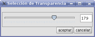
Apply transparency
To manage the rows of the table (add, delete or move) you can use the general table controls located below the table (see the table control description).
Gradient view
The gradient view (which can be accessed by clicking the gradient tab) contains the same information as the tabular view but presented in a different way, and with the possibility to obtain results that are difficult to achieve with the tabular view. The colour bar represents the range of values from minimum on the left to maximum on the right. At the start, the end and on intermediate points on the colour bar are a number of break points with a fixed colour value.

Break point
These break points indicate the colour that will be assigned to the value that falls on that point. A click on a break point will activate the text boxes below the colour bar. These text boxes show the following information about the selected break point:
- Colour: The colour of the break point (which can be modified by clicking on it)
- Class: Label associated with the point. This is the same associated label as in the Class column of the tabular view.
- Value: Pixel value at this break point.
To add a break point, just click below the colour bar. After adding a break point you can modify its information. To remove a break point you can click on it and drag it away.
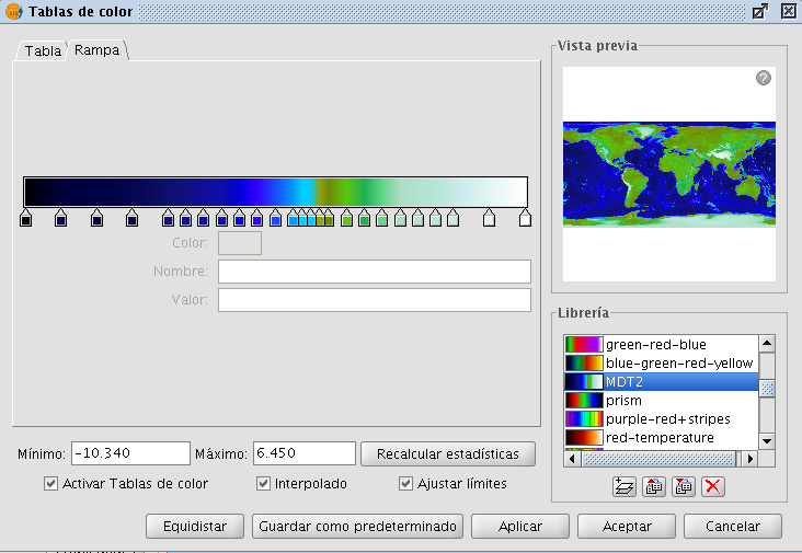
Colour table dialog - Gradient tab
The final result of the gradient will depend on whether the check box labelled as "Interpolated", located below the gradient tab, is ticked or not. This option is available both in the tabular view and the gradient view. When ticked, the transition between one break point colour and the next colour will be gradual. If it is not ticked, the transition will be abrupt. The point where one colour ends and the next colour begins is marked by a diamond-shaped symbol.

Cutoff point
This cutoff point can be moved to the right or the left by clicking and dragging it.
General controls
In the lower part of the dialog are the controls for the tabular and gradient view.
- The text boxes labelled "Minimum" and "Maximum" indicate the minimum and maximum values of the image. We can recalculate these values with the button labelled "Recalc Statistics".
- The check box labelled "Activate colour table" is used to enable or disable the use of colour tables for the current layer.
- Ticking the check box labelled as "Interpolated" will result in a smoother transition between the colours of two ranges of pixel values. This means that instead of assigning a fixed colour to the whole range of pixel values, the RGB colour value of the intermediate pixel values will be the result of an interpolation of the first colour in the range, the last colour in the range and the relative position of the pixel value. If you disable this check box, the transition between colours will be abrupt.
- The check box labelled "Limits adjust" is used to adjust the ranges to the maximum and minimum values of the image. If this is turned off, the colour table will be applied to the whole range of values which is 0 to 255 by default.
- Clicking the button "Middle distance" will result in break points that all hold the same distance between them (they will be equally spread over the colour bar). The first and last values of the range of pixel values will be modified accordingly in the tabular view.
- When clicking the button "Save as Default", the current colour table will be set as the default colour table for this image. The colour table information will be saved as a metadata file (.rmf) with the image, and the next time that the image is loaded in a gvSIG view it will have this colour table associated with it by default.
Library of colour tables
gvSIG provides a list of predefined colour tables to which you can add others that you have built yourself. Located at the lower right part of the Colour table dialog, the colour table libary allows users to scroll through and manage colour tables. The list of colour tables can be displayed in three ways: List, SmallIcon and LargeIcon. The type of display can be changed by right-clicking on the list, after which a drop-down menu appears where you can select the display mode.
List:
Colour table library - List display mode
SmallIcon:
Colour table library - SmallIcon display mode
LargeIcon:
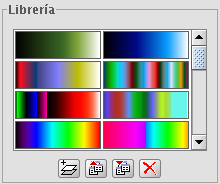
Colour table library - LargeIcon display mode
Below the colour table library are buttons to add, export, import and delete colour tables
- When clicking on the button with the tooltip "New library", a dialog opens which prompts for basic information of the colour table: the name, minimum value, maximum value and the intervals. The default minimum and maximum values are 0 and 255. In principle there is no need to change these values because the colour table is automatically set to the value range of the image to which it is applied. The intervals can be specified by two different methods. The first method is by defining an interval of values, after which the number of intervals is calculated for the whole range of values. The second method is to specify the number of intervals, after which the size of the intervals is calculated automatically.
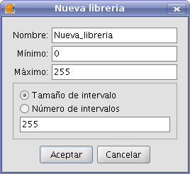
Create new colour table
- To remove colour tables press the button with the tooltip "Delete library". You will be prompted for confirmation before the selected colour table is deleted.
- You can export a colour table in one of the supported formats. Currently, only .rmf y .ggr y .gpl of Gimp are supported.
- You can import a colour table in one of the supported formats. Currently, only .rmf y .ggr y .gpl of Gimp are supported.
Legend in the view and map
The colour table built with this tool will classify the image in ranges of data values. When accepting the colour table dialog settings, this classification is shown in the TOC just below the layer name. For each colour, the corresponding range of values and the associated label, if any, is shown as a legend.
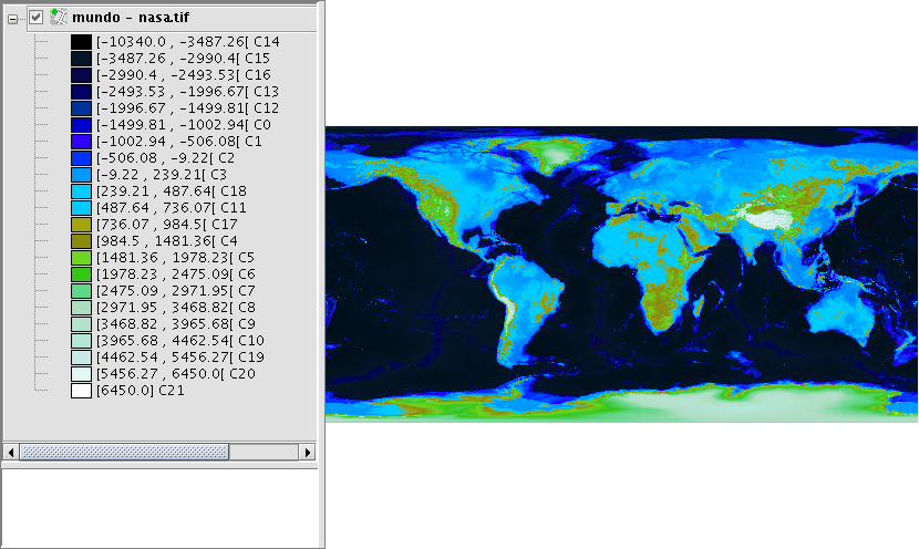
Legend in the ToC according to the colour table of the image
The generated legend can be inserted when preparing a map.
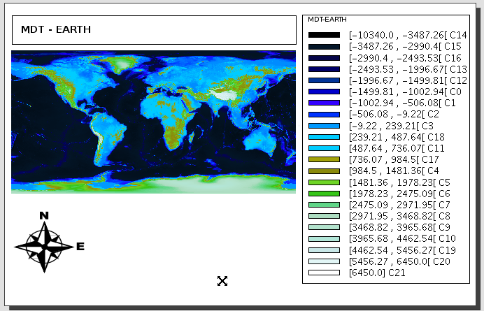
Map with view and legend inserted
Labelling
Introduction
Layer labels are an independent property of the legend that draws the layer geometry. For this reason, labels have been separated from the legend and are treated as entities in their own right. The entity containing the layer labels is a level (containing text) that is drawn above all the other layers in the legend. Note that labels only make sense in certain environments, e.g. vector layers, annotation.
Labelling can be accessed via the new 'Labelling' tab in the 'Layer properties' dialog box (to activate the 'Layer properties' right-click on the active layer in the Table of Contents (ToC) and select 'Properties' or else double-click on the layer name).
Enable labelling in the Layer properties box
There are two general types of labelling:
1- Static labelling (Using attributes from the layer's attribute table)
2- Advanced labelling (User defined)
To activate labelling the 'Enable labelling' option must be checked.
Static labelling
Static labelling automatically creates labels by using values from an existing field in the layer's attribute table. It has been inherited from gvSIG 1.1 and has almost the same functionality that existed before the implementation of Advanced Labelling in the current version of gvSIG.
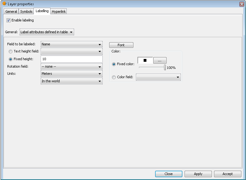
Options for static labelling
These are the options that can be set:
Enable labelling. This enables labelling and displays the layer's labels in the view.
General. For static labelling set this option to 'Label attributes defined in table'.
Field to be labelled. A drop-down list that lets you choose a field in the layer's attribute table that contains values to display as labels.
Text height field option. Select a field in the attribute table that contains the height of each label.
Fixed height option. Enter a fixed value for the size of the labels.
Rotation field. Select a field in the attribute table that denotes the rotation angle of the labels. This must be a numeric field.
Units. Choose the units used for the height values.
Font. Select the font to apply to the labels.
Fixed colour option. Choose a colour for the labels. You can also set the label transparency by using the slider.
Colour field option. Select a field in the attribute table that contains colours.
Advanced Labelling (user defined)
Introduction
User defined labelling provides the user with a great degree of control over the design and placement of labels. It has many more options and is much more powerful than static labelling.
The three different methods of user defined labelling are described below.
Label features in the same way
Choose this option to apply the same label style to all features in the layer, regardless of whether they have been selected or not.
The interface for this labelling option looks like this:
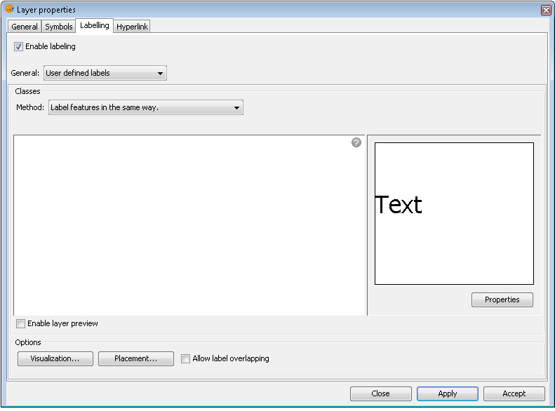
Label all features in the same way
Note the following options, which are explained below:
- Properties
- Visualization
- Placement
It is also possible to preview the labels that have been defined for the layer. These will be applied to the View if the Apply or Accept buttons are clicked.
Label only when the feature is selected
Apply the label setting only to those features that are selected in the View.
This labelling is dynamic, so that if the selection in the View is changed, the View is automatically updated with the labels for the new selection.
The interface for this labelling option is the same as that shown above (Label features in the same way).
Define classes of features and label each differently
With this option the user can create different label classes (through the 'Add' button), assign them a priority for display (using the 'Move up' / 'Move down' buttons to the right of the panel) and label each one separately.
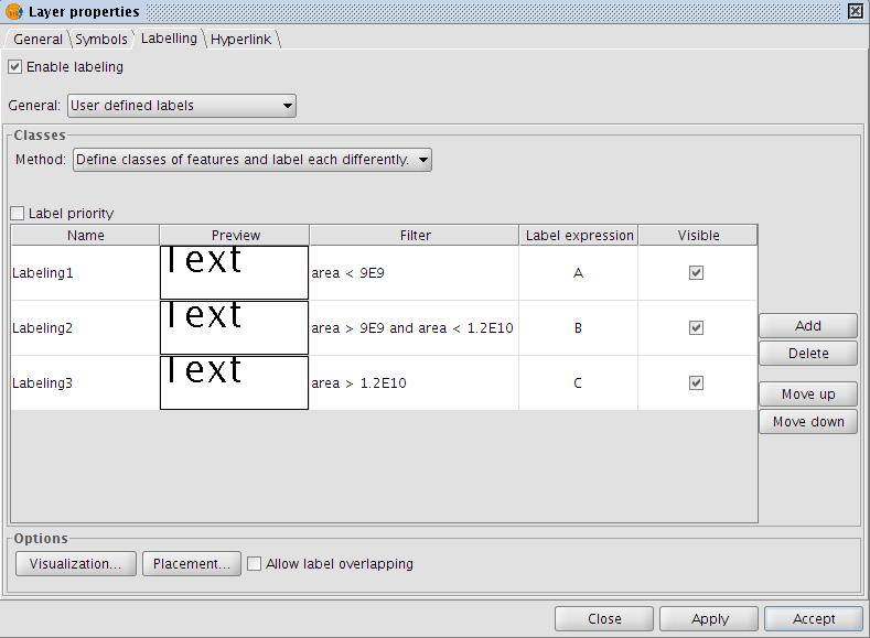
Advanced labelling. Different classes and labelling
The properties for each class can be accessed by double clicking on the relevant class (This brings up a dialog box, which is the same as for the three existing advanced labelling methods).
In other words, the label classes can be configured separately, with different labelling properties and different filters applied to the layer geometry for each class. Keep in mind that the labelling expression uses SLD grammar, while the geometry filter is applied using SQL statements, as defined by GDBMS.
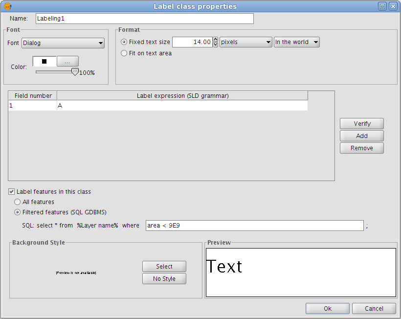
Advanced labelling. Property Configuration
The dialog box below shows how SQL statements can be entered for each of the label classes. These statements act as filters that determine which of the layer's features the class is applied to.
Here is an example of how this SQL filter is used:
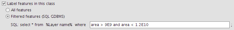
SQL statement for filtering features
Common options
Introduction
Regardless of which advanced labelling method is chosen, there are some options that are common to all three methods. These options provide a great degree of control over the configuration of the labels.
These options are accessible via the buttons on the labelling tab of the Layer properties dialog box and are described below.
Properties
The 'Properties' button provides access to a large number of label options.
Clicking this button opens the dialog box shown in the figure below:
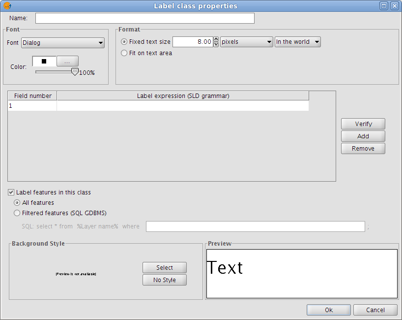
Label class properties
The following properties can be set in this dialog box:
Name
Font type
Font colour
Text size (fixed size or adjusted to fit on text area)
Label expression (one or more)
This is where the actual label is specified. The possibilities are:
- Strings (enclosed in quotes)
- Fields from the attribute table (enclosed in square brackets)
- Mathematical expressions
- Combinations of the above
Label all features / filter features with a SQL statement
The SQL filter allows the user to apply the defined label to certain features only.
Background style
Select a style (picture) as a background for the labels. Clicking the 'Select' button opens the following dialog box:
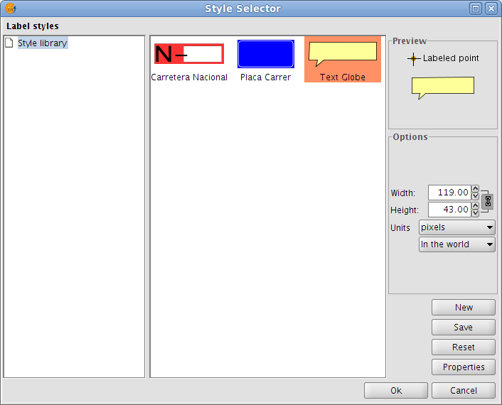
Select a label background style
When gvSIG is installed, the installer automatically creates a directory called 'Styles' in the directory /user/gvSIG/. This is where all the label styles are saved (by clicking the 'Save' button).
Once a label style has been selected, it is possible to modify its properties by clicking the 'Properties' button. This opens a dialog box (shown below) where the user can insert one or more text boxes in which to place the different label expressions that have been created. These text boxes can also be moved or deleted and it is also possible to upload a new image from disk.
Configure the label background style
Note: It is not possible to apply a background style if the label orientation is set to "Following the line" (see the Placement section below).
Placement
Clicking the Placement button opens the Placement properties dialog box where the following properties can be configured: location, orientation, duplicates, etc. The options available in this dialog box will depend on the geometry of the layer in question (point, line or polygon):
Point layer
Placement properties for a point layer
If the layer is a point layer, the following options can be configured:
- Point settings
This options allows the user to place the labels on top of the points, or else to offset them around the points.
In the latter case, the label position can be selected from pre-defined placement configurations, which are accessed by clicking the Change location button. This opens the Placement priorities selector from where existing placement styles can be selected. It is also possible to modify a placement style by highlighting it and clicking the Properties button:
Label priority placement around a point feature
By using the tools on the right and applying them to the location grid on the left it is possible to set the label position priority relative to the point:
1 = High precedence
2 = Normal precedence
3 = Low precedence
0 = Prohibited
- Duplicate labels
Here it is possible to choose between 'Remove duplicate labels' (eliminate any duplicate labels and only draw one label per feature), 'Place one label per feature', and 'Place one label per feature part' (in the case of multipoint features).
Line layer
For line layers the following options are available:
Placement properties for a line layer
- Orientation
The label can be oriented horizontally, parallel or perpendicular to the line, or can be set to follow the line.
- Position
The label can be placed above, on or below the line.
- Location
Place the label at the beginning, middle or end of the line, or at the best position.
- Duplicate labels
The options here are the same as for point layers (described above).
Polygon layer
If the layer is a polygon layer, the Placement properties dialog box provides the following options:
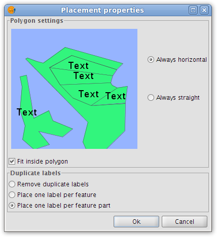
Placement properties for a polygon layer
- Polygon settings
Labels can be set to be always horizontal, or else to follow the orientation of the polygons (always straight). There is also an option for fitting the labels inside the polygons. This last option is used to ensure that labels are placed inside polygons even if they have islands, or are U-shaped.
- Duplicate labels
These options are the same as for point and line layers.
Multigeometry layers
In the case of multigeometry layers (dwg, dxf, gml...) the Placement properties dialog box contains a tab for each of the three geometries (points, lines, polygons). These tabs are identical to those shown above.
Visualisation
Clicking the 'Visualisation' button opens a dialog box which allows configuration of the range of scales at which labels will be shown.
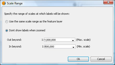
Scale range for a layer's labels
The user can choose to use the same scale range as the feature layer (set under the General tab of the layer properties dialog), or else can specify a scale range at which the labels will be visible (this scale range is independent of the range applied to the geometries of the layer).
In the example shown above, labels in the view are only displayed between the scales of 1:500000 and 1:1000000.
Allow label overlapping
Finally, there is a check box that controls whether labels may overlap or not.
If this box is checked then all labels are drawn, even if they overlap each other. If this box is left unchecked, only non-overlapping labels are drawn and all overlapping labels are eliminated.
Single labelling
In addition to static labelling and user defined advanced labelling, there is a third type of labelling, namely Single Labelling, which can be accessed via the following icon on the toolbar:

Single labelling icon
This type of labelling supplements the existing functionality of annotation layers. In fact, single labelling allows the user to create personalised annotations that have not been possible till now.
The result is an annotation layer, of type shape, plus a file with a .gva extension.
This type of labelling acts only on the geometry that the user has selected in the gvSIG View.
As with advanced labelling, valid label expressions can take on a number of forms:
- Strings
- Fields from the attribute table
- Mathematical expressions
- Combinations of the above
The advantage of Single Labelling over static or user defined labelling, aside from the availability of the many annotation layer labelling options, is that individual labels can be modified and/or moved after they have been created. This is because the labels are in a new, independent layer that can edited just like any other vector layer.
The steps for using this type of labelling are described below:
Configure the annotation properties:
From the main window of this tool, the user can set some basic properties that will apply to the new annotation labels (default annotation properties can be defined in the Annotation properties section of the gvSIG Preferences).
- Font type
- Font style
- Font height
- Font Colour
- Font Rotation
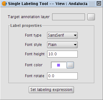
Properties of the annotation being created
Configure the target annotation layer:
As shown in the following dialog box, it is possible to open an existing annotation layer from the hard drive, create a new one in the specified location, or to select one that has already been loaded into the View:
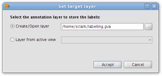
Destination of the annotation layer
Define a labelling expression:
Activate the source layer in the ToC, click the Set labelling expression button and then define an expression in the text box next to the layer name.
An example of this step is shown below:
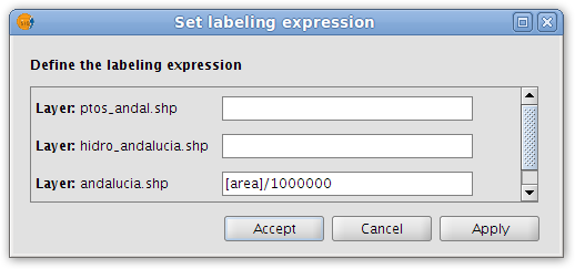
Annotation labelling expression
In the View click on the features that need to be labelled.
In this way, labels are inserted into the View as each of the features is clicked. The labels are drawn according to the label properties set above.
Finally, opening the Layer properties for the annotation layer reveals that a new 'Annotation' tab has been added to the dialog box.
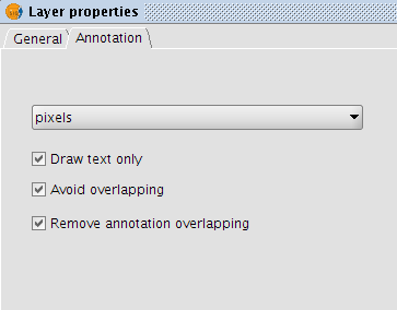
Annotation tab in the Layer properties dialog box
In this tab it is possible to configure a number of annotation options:
- Measurement units (any of the measurement units supported by gvSIG may be selected)
- Draw text only
- Avoid overlapping
- Remove overlapping annotation
Selection tools
Selección de elementos
SELECT ALL
This tool is enabled when one or more vector layers are active in the TOC. The tool selects all the geometries (features/elements) in the active vector layers.
 "Select all" tool enabled if there are active vector layers in the current View.
 "Select all" tool disabled when there are no active vector layers in the current View.
The tool is accessed via the menu:
- View -> Selection -> Select All
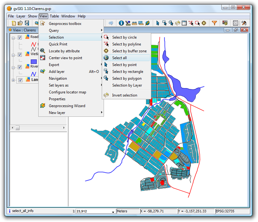
Menu location of Select All tool
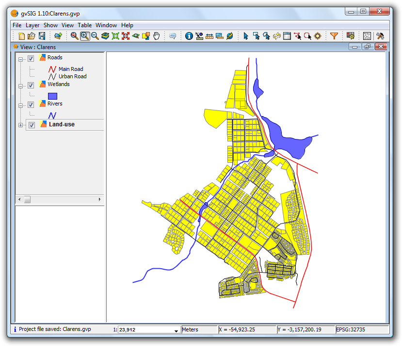
Result of selection
 The tool is not available if the layer is being edited.
SELECT BY POLYLINE
This tool is enabled when there is at least one active vector layer in the TOC.
 "Select by polyline" tool enabled if there are active vector layers in the current View.
 "Select by polyline" tool disabled if there are no active vector layers in the current View.
This tool selects those geometries of the active layers that intersect the polyline defined by the user.
The tool can be accessed in two ways:
- Via the menu: View -> Selection -> Select by polyline
- Via the icon on the toolbar
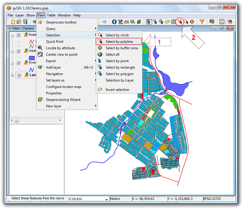
Location of the Select by polyline tool
With the tool selected, move the mouse over the View and enter a series of clicks to define the polyline. Double-click to end the polyline.
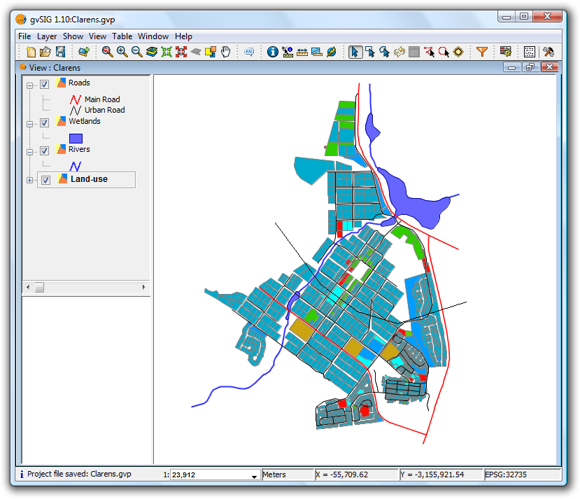
Selection using a polyline
 You can use any mouse button to define the points of the polyline, including the final point.
If another polyline is created while holding down the Ctrl key then the geometries thus selected are added to those already selected. If, while doing this, a previously selected geometry is selected again then it will be deselected.
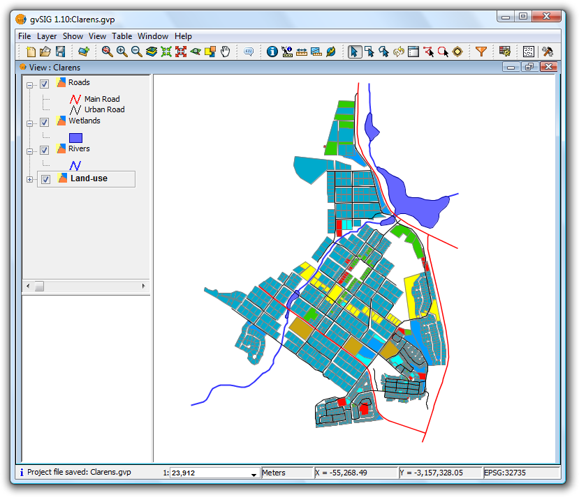
Result of the selection
SELECT BY CIRCLE
This tool is enabled when there are one or more active vector layers in the TOC.
This tool selects geometries (features) of the active layers that intersect the circular area defined by the user.
 "Select by circle" tool enabled if there are active vector layers in the current View.
 "Select by circle" tool disabled if there are no active vector layers in the current View.
The tool can be accessed in two ways:
- Via the menu: View -> Selection -> Select by circle
- Via the icon on the toolbar
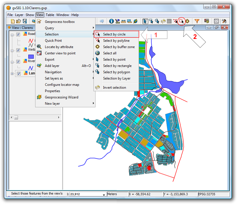
Location of the Select by circle tool
In the View click the mouse at the centre of the circle and then move the mouse outwards to define the size of the circle. Click once to finish drawing the circle.

Selection using a circle
Another circle can be defined while holding down the Ctrl key to add new geometries to those already selected. Previously selected geometries selected again in this manner will be deselected.
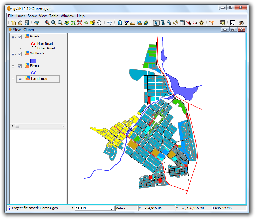
Result of the selection
SELECT BY BUFFER ZONE
This tool is enabled if there is at least one active vector layer in the TOC.
 "Select by buffer zone" tool enabled if there are active vector layers in the current View and these layers have plane coordinates.
 "Select by buffer zone" tool disabled if there are no active vector layers in the current View with plane coordinates.
This tool selects geometries of the active layers that intersect buffer zones around selected geometries.
The tool can be accessed in two ways:
- Via the menu: View -> Selection -> Select by buffer zone
- Via the icon on the toolbar

Location of the Select by buffer zone tool
- Tool requirements
- Vector layers must be active in the TOC
- The selection does not apply to layers with geographical coordinates, only to layers with plane coordinates (e.g. UTM)
- Geometries must be selected in at least one layer
- Configuration panel
When the tool is selected the following configuration panel is displayed:
Configuration options
- Width: width of the buffer zone.
- Unit: units of the buffer zone width.
- Polygon: which side of the polygon to generate the buffer zone:
- Outside: to the outside of the polygon.
- Inside: to the inside of the polygon.
- Line: for line layers the buffer zone will always be towards the outside.
- Point: for point layers the buffer zone will always be towards the outside.
- Multipoint: for multipoint layers the buffer zone will always be towards the outside.
- Multi-layer selection: the selection will apply to all layers that meet the requirements.
- Add buffer zone layers: when selected this option adds the generated buffer zone(s) to the View's TOC.
The new layers are named as follows:
- influence_areas_layername_num
- influence_areas -> prefix to identify this type of layer.
- layername -> name of the layer for which the buffer zone is calculated.
- num -> numerical suffix to identify each new buffer zone layer that is generated, automatically increased for each new zone generated from a single layer, starting from zero.
Example
Let's look at a typical example using the "Select by buffer zone" tool and four layers:
- A shape layer showing "Bird Special Protection Areas" of Castilla y León, obtained from the Ministry of Environment, symbolised with a filled "unique symbol" and with a transparency setting (zepa41):
http://www.mma.es/secciones/biodiversidad/banco_datos/info_disponible/zip/zepa41.zip/
- A shape layer showing "Sites of Community Importance" in Castilla y León, obtained from the Ministry of Environment, and using a unique values symbology:
http://www.mma.es/secciones/biodiversidad/banco_datos/info_disponible/zip/lic41.zip/
- A shape layer shape showing the provinces of Castilla y León, using a unique values symbology.
- A background WMS layer showing hydrographic information, topography, geology, road networks and administrative boundaries in Spain:
WMS Server: http://www.idee.es/wms/PNOA/PNOA/
Layer: PNOA
Style: Default
Format: image/png with transparency and SRS=23030
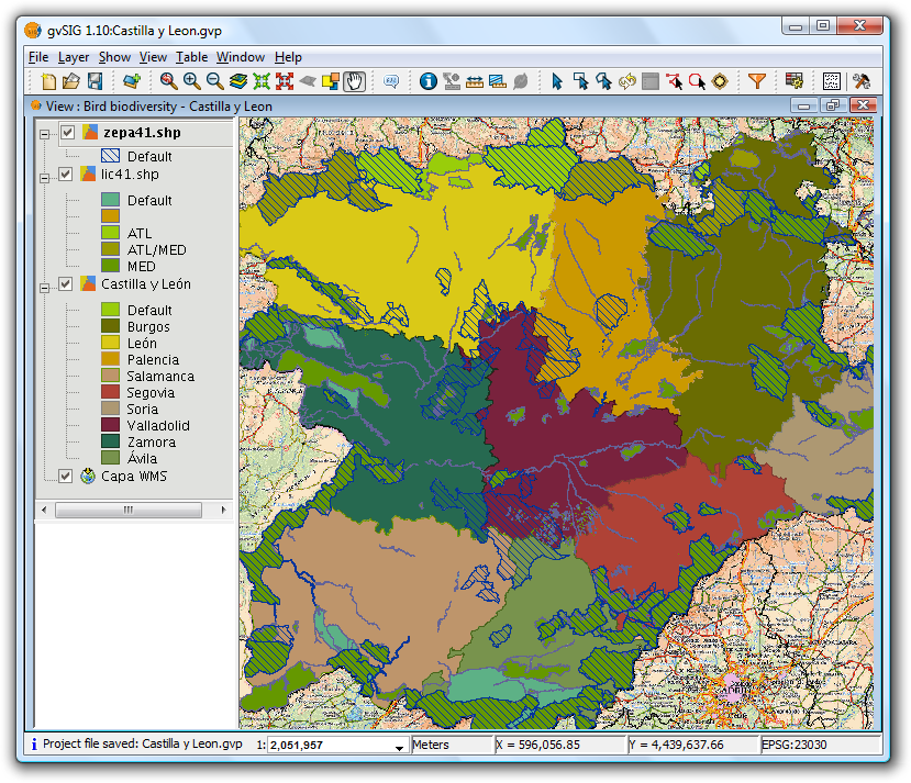
View showing the vector layers, with the Bird Protection Areas layer active
Now select the bird special protection area called "Tierra de Campiñas", which belongs to Valladolid, Ávila and Salamanca. Also select the Site of Community Importance called "Montes Torozos y Páramos de Torquemada – Astudillo" in Valladolid.
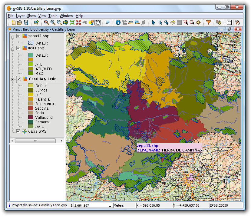
View showing the vector layers, with the provinces layers active
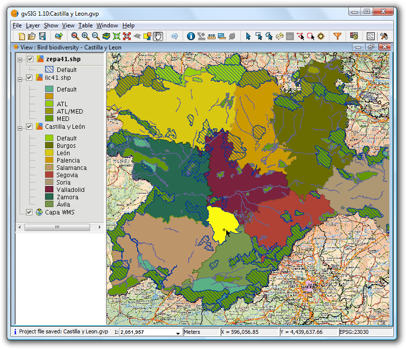
Manual selection of one of the polygons
Make the lic41 layer active
Finally, we want to find the areas of type "lic" and "zepa" close to (up to 15 km) the selected areas so that, for example, they can be taken into account in a future second phase involving work to protect birds.
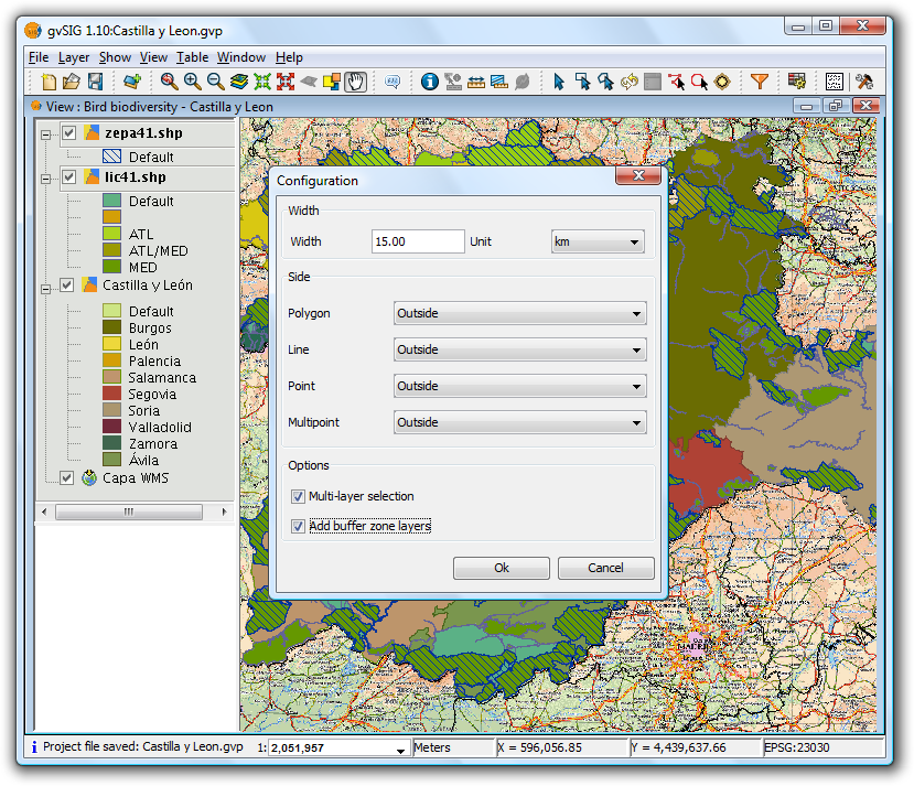
Set options for the buffer zone
The following settings have been applied:
- The zepa41 and lic41 vector layers have been made active.
- Width is set at 15 kilometers.
- The two selected layers are polygon layers, and for this example the buffer zone is set to be outside the polygons.
- Indicate that the selection should be applied to each active layer (Multi-layer selection).
- Finally, add the generated buffer zones as new layers.
The result is shown in the following screenshot. The buffer zones can be turned off so that the selected areas can be seen.
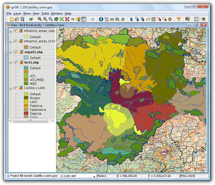
Result of selection by buffer zone
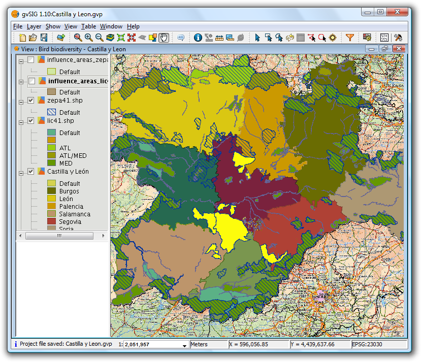
Result with buffer zones switched off
- Details of the process
Click the "Show Details" button below the progress bar to show information on the steps that have been performed, including failures.
Sample output from the above process:
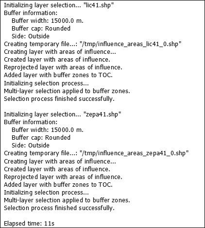
Sample output
Selection is applied to each active layer that meets the requirements.
If the "Multi-layer selection" option is active, then for each buffer zone selections are applied to those layers that also meet the requirements.
If the projection of the layer is not the same as that of the View, an internal reprojection is performed in order to compute the buffer zones. The projection is later restored.
A shape layer is created (one for each active layer that meets the requirements) for storing the buffer zones. The location of each new layer is shown in the line beginning "Creating temporary file".
If the "Add buffer zone layers" option is selected, then the temporary layers are created and added to the TOC, symbolised with a unique symbol and with transparency.
If an active layer is not projected, then the applied selection is discarded.
If a failure occurs, the user is alerted and the selection process is terminated.
 If the process is cancelled, the previous selection state in the affected layers is restored.
Introduction
You can select one or several elements or items by making either a graphic request or an alphanumeric request.
The selected data are shown in the view in the colour you have configured (by default this is yellow).
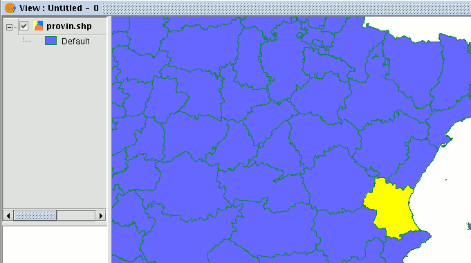
You can access the different ways of selecting elements by going to the tool bar or by going to the “View” menu and then to “Selection” as long as the layer you wish to work with has already been activated in the ToC.
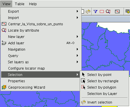
Selecting by point

This is the basic selection method and consists of clicking on the element you wish to select.
Selecting by rectangle

This allows you to select the elements which are partly or wholly located inside a rectangle.
To define the rectangle, place the cursor point over the position you wish to start to draw the rectangle in, left click on the mouse and hold the button down until you have defined the area you wish to select.
Selecting by polygon

This allows you to select elements which are partly or wholly located inside a polygon.
To define this polygon, place the cursor in the part of the view you wish to draw the selection polygon in. Left click on the mouse in the view to add the polygon vertices.
When you have finished, double click on the mouse. All the elements which are located inside the polygon or which intersect with any of its sides will be selected.
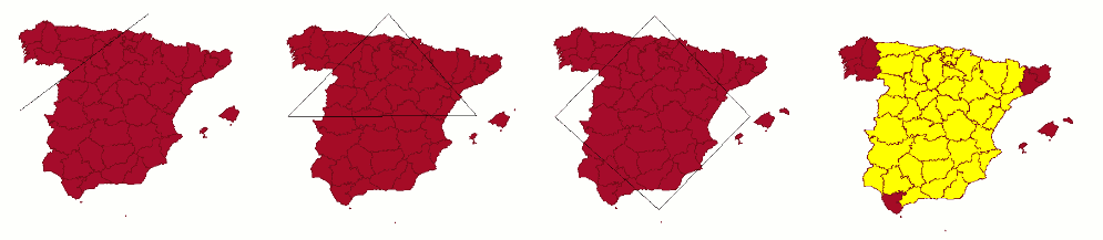
Selecting by layer
You can access this tool by going to the “View” menu then to “Selection” and “Selection by layer”. It allows you to select elements in the active layer based on the selection made in another layer.
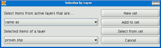
The options available using this tool are:
- 1.New set: This creates a new selection set.
- 2.Add to set: This creates a selection set based on the previous request and the current request.
- 3.Select from set: This creates a selection set from what has already been selected, the current selection request is extracted from the previous one.
An example of how to use this tool consists of selecting the cities and towns of the Valencian Region whose municipal boundaries are affected by flood risks.
We start with a shape file with the areas of the provinces in the Valencian Region which are subject to flood risks.
Then the layer corresponding to all the cities and towns in the Valencian Region is added. Pre-select the full flood risk layer.
We go to the “Selection by layer” tool. Use the “Intersect with” option in the first pull-down menu, “Select items from active layers that are:…”.
Use the “riesgo_inundación_25000_completo” option in the second pull-down menu “Selected items of a layer”.
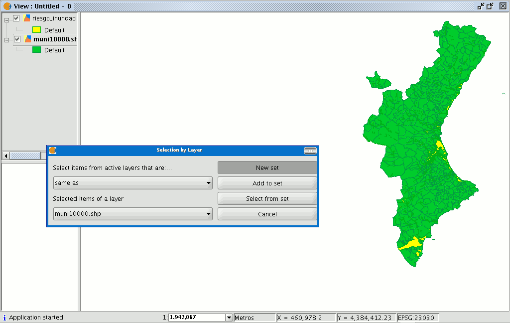
We can now click on “New set” and the layer with the new selection will appear.
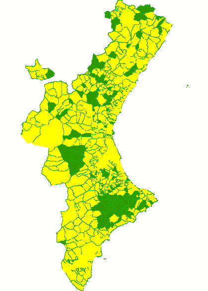
Selecting by attributes
You can access this tool using the following button:

gvSIG allows selections to be made using requests (filters). Selecting elements by attributes allows you to define exactly what you want to select, including several attributes, operators and calculations.
Requests can be made using logical operators, such as “equals” “more than” “different from”, etc.
If you press the “Filter” button in the tool bar, a dialogue window will appear to define your request.
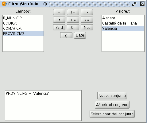
1.Fields: Double click on the field you wish to add to your request from the “Fields” list in the layer.
2.Logical operators: These allow you to insert a logical expression into your request by clicking on them.
3.Values: This shows a list with the different values the selected field has. If you wish to add a value to the request, double click on it.
4.Request: This is the window which represents the request to be made. You can write here directly.
5.Selection buttons: These buttons make the request using:
New set (deletes any previous selections).
Add to set (adds the elements selected by the request to the existing elements).
Select from set (makes the request from the selected elements).
Inverting the selection
When you have made your selection, you can click on the following button in the tool bar

or you can go to the “View” menu then to “Select” and “Invert selection”
and invert the previous selection as shown below.
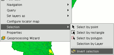
Clearing selection

If you click on this button, the selected element set will once again become empty. You can also access this option by going to the “Layer” menu then to “Clear selection”.
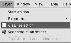
NavTable
¿ Qué es NavTable ?
NavTable is a gvSIG extension to display in an agile way the alphanumeric elements of vectorial layers. It allows seeing the features of an element in a vertical table besides editing, navigating and quick filtering the values of a layer.

NavTable is released under a GPL v3 license. It has been created by CartoLab, the Cartographic Laboratory from University of A Coruña. Feel free to send us comments, suggestions, bug reports, etc.
Listado de características
- Display data from vectorial layers in vertical align
- Edit alphanumeric values (tested with ESRI Shapefile and PostGIS)
- Navigate between elements: next, previous, ...
- Allow to navigate only by selected elements
- Zoom to the elements: manual and automatic
- Allow zoom with fixed scale
- Select and unselect elements
- Alphanumeric editing of values
- Copy attributes from last register or from selected
- Create and drop elements
- Length and area of a element is calculated
- Available in spanish, galician, english and french.
Interfaz
To activate NavTable you must select a vector layer in the gvSIG ToC (Table of Contents) and click the button NavTable  .
.
NavTable interface has the following areas:
- Top: basic adjustments and filter checkboxes.
- Central: view and edit data in each record.
- Bottom: navigate bar, save button and others practical buttons.

NavTable can be used for editing and display alpha-numeric tables, which have no associated geometry. For these cases, NavTable icon in the toolbar will be blue  . The title of the NavTable window for tables without geometry has a '*' to distinguish it from normal tables.
Navegación
NavTable scrolls through the records and features in a friendly way. You will find the navigation bar at the bottom of NavTable's window.

With these buttons you can:
- Go to the first record
- Go to the previous record
- Go to the next record
- Go to the last record
- Go to any record using the box located between the buttons described above. It shows the number of the records you're currently viewing. If you enter a new value here you will see the corresponding record. Next to the position of the box there is a number indicating the total amount of records in the table.
If you are working in the central area of NavTable (click on any row) you can use the buttons “right”or “left”, “home” or “end” to change the record that you want to see.
Selecting elements
If you click on the checkbox "selected" the navigation buttons will work only for features that are previous selected. If a feature is selected, the bottom area of the NavTable Window will be highlighted in yellow. In between parentheses the number of selected records can be seen next to the whole number of records.

In this image you see an example explaining how this function works: record 8 for a layer with 20 records is displayed where 7 records are selected.
If the checkbox "selected" is activated without any selected feature, all records will be shown empty and the box will not display any number. and
 .
.
The option "select" is another interesting tool you can find next to "selected" in the Nav Table menu. If you activate the checkbox next to "select", the attributes you are visualizing will be selected and highlighted in the view. In the case that other features were selected, this option will turn them unselected and will select only the register you are visualizing.
On top of the NavTable Window there is the button "Filter" . If you press it, a dialogue window will appear in which you can define exactly what you want to select (attributes and calculations). If you click on "clear selection"
 all selections will be turned off and no features will be selected.
Zoom to feature
If you click on the zoom button  the feature will be displayed in the center of the view, referring to the record you are working with at that time. The scale of the view will be changed to have a good visualization of the data. In case you are working with a point layer, a scale size will be chosen that allows to see also the surroundings of the point.

With help of the button "always zoom" next to the checkbox "select", Navtable will zoom to each feature referring to the record you are visualizing. If you click on "fixed scale" as well, Navtable will zoom to the feature and display it in the center of the view, but the scale will always remain the same. It is possible to change the scale value introducing a new one in the "scale bar" of gvSIG. This is shown on the buttom right of the gvSIG view, next to where the coordinates are displayed.
Tip: The options "always zoom" or "fixed scale" together with "select" is a very interesting way of navigate through the features of a layer.
Edición
The main new functionality in Navtable is that you don't need to start the editing mode for a layer if you want to edit it. You should follow these steps to edit the table:
- Make double click on the register you wish to work with (or click on the space bar). Now you are in editing modus and you will be able to modify this record.
- Modify the data by entering a new value
- Click on the "save" button
 .
.
After that, the new value will be saved. It's important to consider these special cases if you want to save the edition:
- with boolean fields you can only use true or false (the expression is not case sensitive). If you enter another value, the original one will be saved.
- If you try to save a value into a not appropriate field (for example from type „text“ into type „numerical“), the original value will be written.
- If you want to save an empty text, the default value will be saved. But if the field is from type „string“, the record will be saved with an empty value.
With Navtable it is also possible to use options for advanced editing. For example you can copy and paste records. For that you should select the record you want to copy first and click then on the button "copy selected feature"  . The data will be modified when you click on the button "save".
Removing records
It is possible to delete the record you are visualizing with Navtable if you click on the button "delete feature"  . If this record has an associated geometry feature (graphical element), this one will be also deleted.
Adding records to alphanumerical tables
For tables which aren't associated to a layer, Navtable has this button  . If you click on it, after the last one of the table a new record will appear.
Visualización de nombres largos
As you know, the dbf format doesn't allow field names with more than 10 characters. This limitation could be solved using alias for these fields. This option is also available for layers stored in a geodatabase.
If you wish to use this functionality you will need to create a text file with the same name as the layer in which you want to use "alias" names. Save this text file in the folder "alias" that was created when installing Navtable.
When installing gvSIG, a folder with the name gvSIG will also be created:
On Windows it is usually installed here "C:Documents and Settingsuser"

On GNU/Linux you will find it here: "/home/user/gvSIG"
When installing Navtable, a folder with the Name "Navtable" is saved to the "gvSIG" folders. At the Navtable folder you will find the "Alias" one, where you should save the text file mentioned above.

In this file you can define long names or alias for the field names.
Name_original_field=long_name
It's only necessary to describe a row for the fields you want to define an alias name for. The order of the lines isn't important, that means, you don't need to follow the same sequence like the field's names of the table.
When Navtable is opened, the according "alias" text file will be found automatically. If new names for the fields are available there, Navtable will use these ones instead of the original names.
Example: There is a dbf file with the following fields:

We define an alias text file with the same name as the shape file: Afg_district.alias in this case. In this file we will write the following text:
prov_code=province code
distr_code=district code
This file Afg_district.alias will be saved in the same folder as the file Afg_district.shp. Now we can open the table of this layer with Navtable and can see the following:

Important for Windows:
Windows doesn't show the file extension by default. For this reason for a new alias text file the name of the file will be probably name_layer.alias.txt and Navtable will not be able to read this alias file.
In order to have a correct result for this functionality we recommend you to deactivate the option hide hidden files and folders. You can make this in Windows Explorer: Extras > File Options > View > Advanced Settings > Hidden Files and Folders
Más información sobre NavTable
NavTable is hosted by the OSOR Forge [1]. On this page you can find useful information about the project and also related documents, mailing lists, bug reporting system, etc.
In the section "Future Work" on the project website you will find some of the things we want to incorporate in NavTable in the near future.
| [1] | http://navtable.forge.osor.eu/ |
-----------------------------------
- Se ha producido un error en el documento Navegación , accediendo a la imagen picture_22.png, que probablemente no existe. Se han encontrado las siguientas alternativas [1, 2, 3, 4, ]
- Se ha producido un error en el documento Navegación , accediendo a la imagen picture_14.png, que probablemente no existe. Se han encontrado las siguientas alternativas [1, 2, 3, 4, ]


